
Oracle10g SQL Time-series Tuning
This article is a brief overview of SQL tuning in Oracle10g, with a focus on the new 10g SQL tuning features. The main new features of SQL tuning in Oracle10g include the following:
- Oracle10g now automatically collects and refreshes schema statistics using the dbms_stats package, and histogram collection is now easily automated with dbms_stats
- One common cause of sub-optimal SQL is missing materialized view and indexes, especially function-based indexes. The SQLTuning Advisor and SQLAccess Advisor provide an easy method for identifying and tuning SQL with sub-optimal execution plans.
- SQL Profiles are a great improvement of Optimizer Plan Stability (stored outlines).
- The new dba_hist tables contain a wealth of historical information about historical SQL execution statistics.
- Time-series analysis of object usage within SQL can give us important insights into holistic tuning for SQL statements.
Let’s dive into the most important of all of the Oracle 10g tuning features, the automated Workload Repository, and see how we can perform time-series SQL tuning.
AWR and SQL Tuning
The new Oracle10g AWR tables contain super-useful information about the time-series execution plans for SQL statements and this repository can be used to display details about the frequency of usage for table and indexes. The following are AWR tables for time-series SQL tuning (refer to figure 1):
      • dba_hist_sqlstat
      • dba_hist_sql_summary
      • dba_hist_sql_workarea
      • dba_hist_sql_plan
      • dba_hist_sql_workarea_histogram
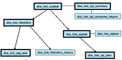
Figure 1: The dba_hist views for SQL tuning.
When we get started with time-series SQL tuning, we have to remember the basic relationships between database objects and SQL statements (refer to figure 2):
- Each SQL statement may generate many access plans — As we know from our discussion of dynamic sampling and dbms_stats, the execution plans for SQL statements will change over time to accommodate changes in the data they access. It’s important to understand how and when a frequently executed SQL statement changes its access plan.
- Each object is accessed by many access plans — In most OLTP systems, tables and indexes show repeating patterns of usage, and we can see clear patterns when we average object access by day-of-the-week and hour-of-the-day.
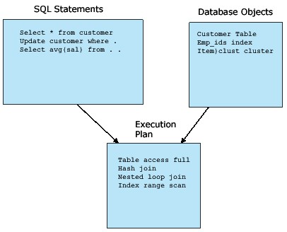
Figure 2: Time-series relationships between SQL and database objects.
As we see, there is a many-to-many relationship between any given SQL statement and the tables they access. Once we understand this fundamental relationship, we can begin to use the AWR tables to perform time-based SQL tuning.
These simple tables represent a revolution in Oracle SQL tuning, and we can now employ time-series techniques to optimizer SQL with better results than ever before. Let’s take a closer look at these views.
dba_hist_sqlstat
This view is very similar to the v$sql view, but it contains important SQL metrics for each snapshot. These include important delta (change) information on disk reads and buffer gets, as well as time-series delta information on application, I/O, and concurrency wait times.
--*************************************************
--   Copyright © 2004 by Rampant TechPress Inc.
--   Free for non-commercial use!
--   To license, e-mail info@rampant.cc
-- ************************************************
col c1 heading ‘Begin|Interval|time’    format a8
col c2 heading ‘SQL|ID’                 format a13
col c3 heading ‘Exec|Delta’             format 9,999
col c4 heading ‘Buffer|Gets|Delta’      format 9,999
col c5 heading ‘Disk|Reads|Delta’       format 9,999
col c6 heading ‘IO Wait|Delta’          format 9,999
col c7 heading ‘Application|Wait|Delta’ format 9,999
col c8 heading ‘Concurrency|Wait|Delta’ format 9,999
break on c1
select
  to_char(s.begin_interval_time,’mm-dd hh24’)  c1,
  sql.sql_id               c2,
  sql.executions_delta     c3,
  sql.buffer_gets_delta    c4,
  sql.disk_reads_delta     c5,
  sql.iowait_delta         c6,
  sql.apwait_delta         c7,
  sql.ccwait_delta         c8
from
   dba_hist_sqlstat        sql,
   dba_hist_snapshot         s
where
   s.snap_id = sql.snap_id
order by
   c1,
   c2
;
Here is a sample of the output. This is very important because we can see the changes in SQL execution over time periods. For each snapshot period, we see the change in the number of times the SQL was executed as well as important performance information about the performance of the statement.
Begin                         Buffer   Disk         Application Concurrency
Interval SQL             Exec   Gets  Reads IO Wait        Wait        Wait
time     ID             Delta  Delta  Delta   Delta       Delta       Delta
-------- ------------- ------ ------ ------ ------- ----------- -----------
10-10 16 0sfgqjz5cs52w     24     72     12       0           3           0
         1784a4705pt01      1    685      6       0          17           0
         19rkm1wsf9axx     10     61      4       0           0           0
         1d5d88cnwxcw4     52    193      4       6           0           0
         1fvsn5j51ugz3      4      0      0       0           0           0
         1uym1vta995yb      1    102      0       0           0           0
         23yu0nncnp8m9     24     72      0       0           6           0
         298ppdduqr7wm      1      3      0       0           0           0
         2cpffmjm98pcm      4     12      0       0           0           0
         2prbzh4qfms7u      1  4,956     19       1          34           5
10-10 17 0sfgqjz5cs52w     30     90      1       0           0           0
         19rkm1wsf9axx     14     88      0       0           0           0
         1fvsn5j51ugz3      4      0      0       0           0           0
         1zcdwkknwdpgh      4      4      0       0           0           0
         23yu0nncnp8m9     30     91      0       0           0           5
         298ppdduqr7wm      1      3      0       0           0           0
         2cpffmjm98pcm      4     12      0       0           0           0
         2prbzh4qfms7u      1  4,940     20       0           0           0
         2ysccdanw72pv     30     60      0       0           0           0
         3505vtqmvvf40      2    321      5       1           0           0
This report is especially useful because we can track the logical I/O (buffer gets) vs. physical I/O for each statement over time; this provides important information about the behavior of the SQL statement.
This output gives us a quick overview of the top SQL statements during any AWR snapshot period and shows how their behavior has changed since the last snapshot period. Detecting changes in the behavior of commonly executed SQL statements is the key to time-series SQL tuning.
Note that we can easily add a WHERE clause to the above script and plot the I/O changes over time:
< awr_sqlstat_deltas_detail.sql

--*************************************************
--   Copyright © 2004 by Rampant TechPress Inc.
--   Free for non-commercial use!
--   To license, e-mail info@rampant.cc
-- ************************************************

col c1 heading ‘Begin|Interval|time’    format a8
col c2 heading ‘Exec|Delta’             format 999,999
col c3 heading ‘Buffer|Gets|Delta’      format 999,999
col c4 heading ‘Disk|Reads|Delta’       format 9,999
col c5 heading ‘IO Wait|Delta’          format 9,999
col c6 heading ‘App|Wait|Delta’         format 9,999
col c7 heading ‘Cncr|Wait|Delta’        format 9,999
col c8 heading ‘CPU|Time|Delta’         format 999,999
col c9 heading ‘Elpsd|Time|Delta’       format 999,999


accept sqlid prompt ‘Enter SQL ID: ‘

ttitle ‘time series execution for|&sqlid’

break on c1

select
  to_char(s.begin_interval_time,’mm-dd hh24’)  c1,
  sql.executions_delta     c2,
  sql.buffer_gets_delta    c3,
  sql.disk_reads_delta     c4,
  sql.iowait_delta         c5,
  sql.apwait_delta         c6,
  sql.ccwait_delta         c7,
  sql.cpu_time_delta       c8,
  sql.elapsed_time_delta   c9
from
   dba_hist_sqlstat        sql,
   dba_hist_snapshot         s
where
   s.snap_id = sql.snap_id
and
   sql_id = ‘&sqlid’
order by
   c1
;
Here we can see the changes to the execution of a frequently used SQL statement and how its behavior changes over time:
Begin               Buffer   Disk            App   Cncr      CPU    Elpsd
Interval     Exec     Gets  Reads IO Wait   Wait   Wait     Time     Time
time        Delta    Delta  Delta   Delta  Delta  Delta    Delta    Delta
-------- -------- -------- ------ ------- ------ ------ -------- --------
10-14 10      709    2,127      0       0      0      0  398,899  423,014
10-14 11      696    2,088      0       0      0      0  374,502  437,614
10-14 12      710    2,130      0       0      0      0  384,579  385,388
10-14 13      693    2,079      0       0      0      0  363,648  378,252
10-14 14      708    2,124      0       0      0      0  373,902  373,902
10-14 15      697    2,091      0       0      0      0  388,047  410,605
10-14 16      707    2,121      0       0      0      0  386,542  491,830
10-14 17      698    2,094      0       0      0      0  378,087  587,544
10-14 18      708    2,124      0       0      0      0  376,491  385,816
10-14 19      695    2,085      0       0      0      0  361,850  361,850
10-14 20      708    2,124      0       0      0      0  368,889  368,889
10-14 21      696    2,088      0       0      0      0  363,111  412,521
10-14 22      709    2,127      0       0      0      0  369,015  369,015
10-14 23      695    2,085      0       0      0      0  362,480  362,480
10-15 00      709    2,127      0       0      0      0  368,554  368,554
10-15 01      697    2,091      0       0      0      0  362,987  362,987
10-15 02      696    2,088      0       0      0      2  361,445  380,944
10-15 03      708    2,124      0       0      0      0  367,292  367,292
10-15 04      697    2,091      0       0      0      0  362,279  362,279
10-15 05      708    2,124      0       0      0      0  367,697  367,697
10-15 06      696    2,088      0       0      0      0  361,423  361,423
10-15 07      709    2,127      0       0      0      0  374,766  577,559
10-15 08      697    2,091      0       0      0      0  364,879  410,328
In the preceding listing, we see how the number of executions varies over time.
But AWR has lots more useful information. Let’s now look at the dba_hist_sql_plan table.
dba_hist_sql_plan
The dba_hist_sql_plan table contains time-series data about each object (table, index, view) involved in the query. The important columns include the cost, cardinality, cpu_cost, io_cost, and temp_space required for the object. The sample query below retrieves SQL statements that have high query execution cost identified by Oracle optimizer.
But there is a lot more information in dba_hist_sql_plan that is useful. The query below will extract important costing information for all objects involved in each query (SYS objects are not counted).
< awr_sql_object_char.sql
--*************************************************
-- Copyright © 2004 by Rampant TechPress Inc.
-- Free for non-commercial use!
-- To license, e-mail info@rampant.cc
-- ************************************************
col c1 heading ‘Owner’              format a13
col c2 heading ‘Object|Type’        format a15
col c3 heading ‘Object|Name’        format a25
col c4 heading ‘Average|CPU|Cost’   format 9,999,999
col c5 heading ‘Average|IO|Cost’    format 9,999,999
break on c1 skip 2
break on c2 skip 2
select
  p.object_owner    c1,
  p.object_type     c2,
  p.object_name     c3,
  avg(p.cpu_cost)   c4,
  avg(p.io_cost)    c5
from
  dba_hist_sql_plan p
where
        p.object_name is not null
    and
        p.object_owner <> 'SYS'
group by
  p.object_owner,
  p.object_type,
  p.object_name
order by
  1,2,4 desc
;
Here is a sample of the output. Here we see the average CPU and I/O costs for all objects that participate in queries, over time periods.
                                                           Average    Average
              Object          Object                           CPU         IO
Owner         Type            Name                            Cost       Cost
------------- --------------- ------------------------- ---------- ----------
OLAPSYS       INDEX           CWM$CUBEDIMENSIONUSE_IDX         200          0
OLAPSYS       INDEX (UNIQUE)  CWM$DIMENSION_PK
OLAPSYS                       CWM$CUBE_PK                    7,321          0
OLAPSYS                       CWM$MODEL_PK                   7,321          0
OLAPSYS       TABLE           CWM$CUBE                       7,911          0
OLAPSYS                       CWM$MODEL                      7,321          0
OLAPSYS                       CWM2$CUBE                      7,121          2
OLAPSYS                       CWM$CUBEDIMENSIONUSE             730          0
PERFSTAT      INDEX (UNIQUE)  STATS$TIME_MODEL_STATNAME     39,242          2
PERFSTAT                      STATS$SYSSTAT_PK              21,564          2
PERFSTAT                      STATS$SGASTAT_U               21,442          2
PERFSTAT                      STATS$SQL_SUMMARY_PK          16,842          2
PERFSTAT                      STATS$SQLTEXT_PK              14,442          1
PERFSTAT                      STATS$IDLE_EVENT_PK            8,171          0
PERFSTAT      TABLE           STATS$SYSSTAT              5,571,375         24
PERFSTAT                      STATS$FILE_HISTOGRAM       1,373,396          5
PERFSTAT                      STATS$SYSTEM_EVENT           996,571          6
PERFSTAT                      STATS$LATCH                  462,161          5
PERFSTAT                      STATS$SQL_SUMMARY            440,038          7
PERFSTAT                      STATS$PARAMETER              361,439          5
PERFSTAT                      STATS$FILESTATXS             224,227          3
PERFSTAT                      STATS$WAITSTAT               144,554          3
PERFSTAT                      STATS$TEMP_HISTOGRAM         126,304          3
PERFSTAT                      STATS$LIBRARYCACHE           102,846          3
PERFSTAT                      STATS$TEMPSTATXS              82,762          3
PERFSTAT                      STATS$SGASTAT                 51,807          5
PERFSTAT                      STATS$SQLTEXT                 17,781          2
PERFSTAT                      STATS$SQL_PLAN_USAGE               0          2
SPV           INDEX (UNIQUE)  WSPV_REP_PK                    7,321          0
SPV                           SPV_ALERT_DEF_PK               7,321          0
SPV           TABLE           WSPV_REPORTS                 789,052         28
SPV                           SPV_MONITOR                   54,092          3
SPV                           SPV_SAVED_CHARTS              38,337          3
SPV                           SPV_DB_LIST                   37,487          3
SPV                           SPV_SCHED                     35,607          3
SPV                           SPV_FV_STAT                   35,607          3
SPV                           SPV_ALERT_DEF                 15,868          1
SPV                           SPV_BASELINES                  7,121          2
SPV                           SPV_ALERT_HISTORY              7,121          2
SPV                           SPV_STORED_SNAP_RANGES         7,121          2
We can now easily change this script to allow us to enter a table name and see changes in access details over time:
< awr_sql_object_char_detail.sql
--*************************************************
-- Copyright © 2004 by Rampant TechPress Inc.
-- Free for non-commercial use!
-- To license, e-mail info@rampant.cc
-- ************************************************
accept tabname prompt ‘Enter Table Name:’
col c0 heading ‘Begin|Interval|time’ format a8
col c1 heading ‘Owner’               format a10
col c2 heading ‘Object|Type’         format a10
col c3 heading ‘Object|Name’         format a15
col c4 heading ‘Average|CPU|Cost’    format 9,999,999
col c5 heading ‘Average|IO|Cost’     format 9,999,999
break on c1 skip 2
break on c2 skip 2
select
  to_char(sn.begin_interval_time,'mm-dd hh24') c0,
  p.object_owner                               c1,
  p.object_type                                c2,
  p.object_name                                c3,
  avg(p.cpu_cost)                              c4,
  avg(p.io_cost)                               c5
from
  dba_hist_sql_plan p,
  dba_hist_sqlstat  st,
  dba_hist_snapshot sn
where
  p.object_name is not null
and
    p.object_owner <> 'SYS'
and
    p.object_name = 'STATS$SYSSTAT'
and
  p.sql_id = st.sql_id
and
  st.snap_id = sn.snap_id
group by
  to_char(sn.begin_interval_time,'mm-dd hh24'),
  p.object_owner,
  p.object_type,  p.object_name
order by
  1,2,3 desc
;
Here we can see changes in the table’s access patterns over time, a very useful feature:
Begin                                             Average    Average
Interval            Object     Object                 CPU         IO
time     Owner      Type       Name                  Cost       Cost
-------- ---------- ---------- --------------- ---------- ----------
10-25 17 PERFSTAT   TABLE      STATS$SYSSTAT       28,935          3
10-26 15 PERFSTAT              STATS$SYSSTAT       28,935          3
10-27 18 PERFSTAT              STATS$SYSSTAT    5,571,375         24
10-28 12 PERFSTAT              STATS$SYSSTAT       28,935          3
Now that we see the important table structures, let’s examine how we can get spectacular reports from this AWR data.
Viewing Table and Index Access with AWR
One of the problems in Oracle9i was the single bit-flag that was used to monitor index usage. You could set the flag with the alter index xxx monitoring usage command, and see if the index was accessed by querying the v$object_usage view.
As we recall, the goal of any index access is to use the most selective index for a query, the one that produces the smallest number of rows. The Oracle data dictionary is usually quite good at this, but it is up to you to define the index. Missing function-based indexes are a common source of sub-optimal SQL execution because Oracle will not use an indexed column unless the WHERE clause matches the index column exactly.
Let’s look at the awr_sql_index.sql script that exposes the cumulative usage of database indexes:
< awr_sql_index.sql
--*************************************************
-- Copyright © 2004 by Rampant TechPress Inc.
-- Free for non-commercial use!
-- To license, e-mail info@rampant.cc
-- ************************************************
col c0 heading ‘Begin|Interval|time’ format a8
col c1 heading ‘Index|Name’          format a20
col c2 heading ‘Disk|Reads’          format 99,999,999
col c3 heading ‘Rows|Processed’      format 99,999,999
select
  to_char(s.begin_interval_time,'mm-dd hh24')  c0,
  p.object_name               c1,
  sum(t.disk_reads_total)     c2,
  sum(t.rows_processed_total) c3
from
       dba_hist_sql_plan p,
       dba_hist_sqlstat  t,
       dba_hist_snapshot s
where
       p.sql_id = t.sql_id
   and
       t.snap_id = s.snap_id
   and
       p.object_type like '%INDEX%'
group by
       to_char(s.begin_interval_time,'mm-dd hh24'),
       p.object_name
order by
       c0,c1,c2 desc
;
Here is a sample of the output:
Begin
Interval Index                       Disk        Rows
time     Name                       Reads   Processed
-------- -------------------- ----------- -----------
10-14 12 I_CACHE_STATS_1                          114
10-14 12 I_COL_USAGE$                 201       8,984
10-14 12 I_FILE1                        2           0
10-14 12 I_IND1                        93         604
10-14 12 I_JOB_NEXT                     1     247,816
10-14 11 I_KOPM1                        4       2,935
10-14 11 I_MON_MODS$_OBJ               12      28,498
10-14 11 I_OBJ1                    72,852         604
10-14 11 I_PARTOBJ$                    93         604
10-14 11 I_SCHEDULER_JOB2               4           0
1014 11 SYS_C002433                  302       4,629
10-14 11 SYS_IOT_TOP_8540               0      75,544
10-14 11 SYS_IOT_TOP_8542               1       4,629
10-14 11 WRH$_DATAFILE_PK               2           0
10-14 10 WRH$_SEG_STAT_OBJ_PK          93         604
10-14 10 WRH$_TEMPFILE_PK                           0
10-14 10 WRI$_ADV_ACTIONS_PK           38       1,760
You can also use the dba_hist_sql_plan table to gather counts about the frequency of participation of objects inside queries.
< awr_sql_object_freq.sql
--*************************************************
-- Copyright © 2004 by Rampant TechPress Inc.
-- Free for non-commercial use!
-- To license, e-mail info@rampant.cc
-- ************************************************
col c1 heading ‘Object|Name’         format a30
col c2 heading ‘Operation’           format a15
col c3 heading ‘Option’              format a15
col c4 heading ‘Object|Count’        format 999,999
break on c1 skip 2
break on c2 skip 2
select
  p.object_name c1,
  p.operation   c2,
  p.options     c3,
  count(1)      c4
from
  dba_hist_sql_plan p,
  dba_hist_sqlstat s
where
      p.object_owner <> 'SYS'
  and
      p.sql_id = s.sql_id
group by
  p.object_name, p.operation, p.options
order by
  1,2,3;
Here is the output that shows each table and the resulting access method totals:
Object                                                           Object
Name                           Operation       Option            Count
------------------------------ --------------- --------------- --------
CUSTOMER                       TABLE ACCESS    FULL                 305

CUSTOMER  _CHECK               INDEX           RANGE SCAN             2

CUSTOMER_ORDERS                TABLE ACCESS    BY INDEX ROWID       311
CUSTOMER_ORDERS                                FULL                   1

CUSTOMER_ORDERS_PRIMARY        INDEX           FULL SCAN              2
CUSTOMER_ORDERS_PRIMARY                        UNIQUE SCAN          311
AVAILABILITY_PRIMARY_KEY                       RANGE SCAN             4
CON_UK                                         RANGE SCAN             3
CURRENT_SEVERITY_PRIMARY_KEY                   RANGE SCAN             1

CWM$CUBE                       TABLE ACCESS    BY INDEX ROWID         2
CWM$CUBEDIMENSIONUSE                           BY INDEX ROWID         2


CWM$CUBEDIMENSIONUSE_IDX       INDEX           RANGE SCAN             2
CWM$CUBE_PK                                    UNIQUE SCAN            2
CWM$DIMENSION_PK                               FULL SCAN              2

MGMT_INV_VERSIONED_PATCH       TABLE ACCESS    BY INDEX ROWID         3
MGMT_JOB                                       BY INDEX ROWID       458
MGMT_JOB_EMD_STATUS_QUEUE                      FULL                 181
MGMT_JOB_EXECUTION                             BY INDEX ROWID       456

MGMT_JOB_EXEC_IDX01            INDEX           RANGE SCAN           456

MGMT_JOB_EXEC_SUMMARY          TABLE ACCESS    BY INDEX ROWID       180

MGMT_JOB_EXEC_SUMM_IDX04       INDEX           RANGE SCAN           180


MGMT_JOB_HISTORY               TABLE ACCESS    BY INDEX ROWID         1

MGMT_JOB_HIST_IDX01            INDEX           RANGE SCAN             1
MGMT_JOB_PK                                    UNIQUE SCAN          458


MGMT_METRICS                   TABLE ACCESS    BY INDEX ROWID       180
Using the previous output, we are able to easily monitor object participation (especially indexes) in the SQL queries and the mode in which an object was accessed by Oracle.
We can also count specific access methods and see how they change over time. This is especially important for large-table full-table scans (LTFTS) because they are a common symptom of sub-optimal execution plans (i.e., missing indexes).
Once we are assured that the large-table, full-table scans are legitimate, we must know the times when they are executed so that we can implement selective parallel query, depending on the existing CPU consumption on the server (as we know, OPQ drives up CPU consumption, and should be invoked only when the server can handle the additional load).
< awr_full_table_scans.sql
--*************************************************
-- Copyright © 2004 by Rampant TechPress Inc.
-- Free for non-commercial use!
-- To license, e-mail info@rampant.cc
-- ************************************************
ttile ‘Large Tabe Full-table scans|Per Snapshot Period’
col c1 heading ‘Begin|Interval|time’ format a20
col c4 heading ‘FTS|Count’           format 999,999
break on c1 skip 2
break on c2 skip 2
select
  to_char(sn.begin_interval_time,'yy-mm-dd hh24')  c1,
  count(1)                                         c4
from
   dba_hist_sql_plan p,
   dba_hist_sqlstat  s,
   dba_hist_snapshot sn,
   dba_segments      o
where
   p.object_owner <> 'SYS'
and
   p.object_owner = o.owner
and
   p.object_name = o.segment_name
and
   o.blocks > 1000
and
   p.operation like '%TABLE ACCESS%'
and
   p.options like '%FULL%'
and
   p.sql_id = s.sql_id
and
   s.snap_id = sn.snap_id
group by
  to_char(sn.begin_interval_time,'yy-mm-dd hh24')
order by
  1;
From the following output, we see overall total counts for full-tables experience large-table full-table scans. These scans may be due to a missing index.
Begin
Interval                FTS
time                    Count
-------------------- --------
04-10-18 11                 4
04-10-21 17                 1
04-10-21 23                 2
04-10-22 15                 2
04-10-22 16                 2
04-10-22 23                 2
04-10-24 00                 2
04-10-25 00                 2
04-10-25 10                 2
04-10-25 17                 9
04-10-25 18                 1
04-10-25 21                 1
04-10-26 12                 1
04-10-26 13                 3
04-10-26 14                 3
04-10-26 15                11
04-10-26 16                 4
04-10-26 17                 4
04-10-26 18                 3
04-10-26 23                 2
04-10-27 13                 2
04-10-27 14                 3
04-10-27 15                 4
04-10-27 16                 4
04-10-27 17                 3
04-10-27 18                17
04-10-27 19                 1
04-10-28 12                22
04-10-28 13                 2
04-10-29 13                 9
You can easily plot this data and see the trend for your database (refer to figure 3):
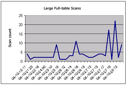
Figure 3: Trends of large-table full-table scans.
Here is an amazing script that will show you the access patterns of usage over time. If you really want to “know your system,” understanding how SQL accesses the tables and indexes in your database can provide you with amazing insights. As we know, the optimal instance configuration for large-table full-table scans is quite different then the configuration for an OLTP databases, and this handy report will quickly identify changes in table access patterns.
< awr_sql_scan_sums.sql


--*************************************************
-- Copyright © 2004 by Rampant TechPress Inc.
-- Free for non-commercial use!
-- To license, e-mail info@rampant.cc
-- ************************************************

col c1 heading ‘Begin|Interval|Time’          format a20
col c2 heading ‘Large|Table|Full Table|Scans’ format 999,999
col c3 heading ‘Small|Table|Full Table|Scans’ format 999,999
col c4 heading ‘Total|Index|Scans’            format 999,999

select
  f.c1  c1,
  f.c2  c2,
  s.c2  c3,
  i.c2  c4
from
(
select
  to_char(sn.begin_interval_time,'yy-mm-dd hh24')  c1,
  count(1)                           c2
from
  dba_hist_sql_plan p,
   dba_hist_sqlstat  s,
   dba_hist_snapshot sn,
   dba_segments      o
where
   p.object_owner <> 'SYS'
and
   p.object_owner = o.owner
and
   p.object_name = o.segment_name
and
   o.blocks > 1000
and
   p.operation like '%TABLE ACCESS%'
and
   p.options like '%FULL%'
and
   p.sql_id = s.sql_id
and
   s.snap_id = sn.snap_id
group by
  to_char(sn.begin_interval_time,'yy-mm-dd hh24')
order by
1 ) f,
(
select
  to_char(sn.begin_interval_time,'yy-mm-dd hh24')  c1,
  count(1)                           c2
from
   dba_hist_sql_plan p,
   dba_hist_sqlstat  s,
   dba_hist_snapshot sn,
   dba_segments      o
where
   p.object_owner <> 'SYS'
and
   p.object_owner = o.owner
and
   p.object_name = o.segment_name
and
   o.blocks < 1000
and
   p.operation like '%INDEX%'
and
   p.sql_id = s.sql_id
and
   s.snap_id = sn.snap_id
group by
  to_char(sn.begin_interval_time,'yy-mm-dd hh24')
order by
1 ) s,
(
select
  to_char(sn.begin_interval_time,'yy-mm-dd hh24')  c1,
  count(1)                           c2
from
   dba_hist_sql_plan p,
   dba_hist_sqlstat  s,
   dba_hist_snapshot sn
where
   p.object_owner <> 'SYS'
and
  p.operation like '%INDEX%'
and
   p.sql_id = s.sql_id
and
   s.snap_id = sn.snap_id
group by
  to_char(sn.begin_interval_time,'yy-mm-dd hh24')
order by
1 ) i
where
      f.c1 = s.c1
   and
      f.c1 = i.c1
;
The sample output looks like:
Begin                     Table      Table    Total
Interval             Full Table Full Table    Index
Time                      Scans      Scans    Scans
-------------------- ---------- ---------- --------
04-10-22 15                   2         19       21
04-10-22 16                              1        1
04-10-25 10                             18       20
04-10-25 17                   9         15       17
04-10-25 18                   1         19       22
04-10-25 21                             19       24
04-10-26 12                             23       28
04-10-26 13                   3         17       19
04-10-26 14                             18       19
04-10-26 15                  11          4        7
04-10-26 16                   4         18       18
04-10-26 17                             17       19
04-10-26 18                   3         17       17
04-10-27 13                   2         17       19
04-10-27 14                   3         17       19
04-10-27 15                   4         17       18
04-10-27 16                             17       17
04-10-27 17                   3         17       20
04-10-27 18                  17         20       22
04-10-27 19                   1         20       26
04-10-28 12                  22         17       20
04-10-28 13                   2         17       17
04-10-29 13                   9         18       19
This is a very important report because it shows you how Oracle is accessing data over time periods. This is especially important because it shows when the database processing modality shifts between OLTP (first_rows index access) to a batch reporting mode (all_rows full scans).
Of course, in a really busy database, you may have concurrent OLTP index access and full-table scans for reports, and it is your job to know the specific times when you shift table access modes, as well as which tables experience the changes.
Conclusion
This is just a taste of the researching that I’m doing for my upcoming book, Oracle 10g Tuning by Rampant TechPress, due out in March 2004. The ability to see SQL executions over time will revolutionize Oracle tuning and allow Oracle professionals to finally understand the dynamic nature of their database.
In later installments, I’ll show you even more advanced time-series SQL tuning scripts, and be sure to check out my DBAzine.com Webinar on “Oracle 10g Time Series SQL Tuning Techniques.”
--
Donald K. Burleson is one of the world’s top Oracle Database experts with more than 20 years of full-time DBA experience. He specializes in creating database architectures for very large online databases and he has worked with some of the world’s most powerful and complex systems. A former Adjunct Professor, Don Burleson has written 15 books, published more than 100 articles in national magazines, serves as Editor-in-Chief of Oracle Internals and edits for Rampant TechPress. Don is a popular lecturer and teacher and is a frequent speaker at Oracle Openworld and other international database conferences. Don’s Web sites include DBA-Oracle, Remote-DBA, Oracle-training, remote support and remote DBA.
Contributors : Donald K. Burleson
Last modified 2005-06-22 12:06 AM