Tuning a single SQL query is an enormously important topic. Before going into production virtually every system would expose some statements that require tuning. In this article, we'll explore several Oracle 9.2 improvements that make life of performance analyst easier.

Access and Filter Predicates

Syntactically, SQL query consists of three fundamental parts:

•  list of columns,
• a list of tables, and
• a where clause.

The where clause is a logical formula that can be further decomposed into predicates connected by Boolean connectives. For example, the where clause of

select empno, sal from emp e, dept d
where e.deptno = d.deptno and dname = 'ACCOUNTING'

is a conjunction of dname = 'ACCOUNTING' single table predicate and e.deptno = d.deptno join predicate.

Arguably, predicate handling is the heart of SQL optimization: predicates could be transitively added, rewritten using Boolean Algebra laws, moved around at SQL Execution Plan, and so on. In our simplistic example, the single table predicate is applied either to index or table scan plan nodes, while join predicate could also be applied to the join node. Unfortunately, despite their significance, Oracle Execution Plan facility didn't show predicates until version 9.2. (although, experts had an option of running 10060 event trace).

In the latest release PLAN_TABLE (together with its runtime sibling V$SQL_PLAN) acquired two new columns:

ACCESS_PREDICATES      VARCHAR(4000)
FILTER_PREDICATES      VARCHAR(4000)

In our example, the plan

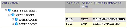
now explicitly shows us that dname = 'ACCOUNTING' single table predicate is filtering rows during the outer table scan, while e.deptno = d.deptno join predicate is applied during each inner table scan.

I found it convenient to apply a little bit of GUI "sugarcoating" and display the plan as

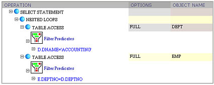
especially in the cases where predicates are complex. Consider an example with nested subquery:

select empno, sal from emp e
where sal in (select max(sal) from emp ee)

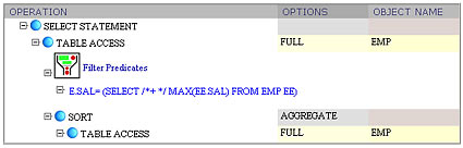
Here the filter predicate contains the whole subquery. Again, predicate visualization helps understanding how the plan is executed. Since the subquery is not correlated, it can be evaluated once only. Two innermost plan nodes are responsible for execution of nested subquery. Then, the emp e table from the outer query block is scanned, and only the rows that meet filter condition remain in the result set.

My next example demonstrates predicate transitivity:

select e.empno, d.dname from emp e, dept d
where e.deptno = d.deptno and e.deptno = 10

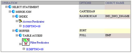
From the plan, it becomes obvious that the optimizer chose a Cartesian Product because it considered worthwhile dropping join predicate e.deptno = d.deptno and using the derived d.deptno = 10 predicate instead.

In this example, we also see the Access Predicates in action for the first time. If we add one more predicate

select e.empno, d.dname from emp e, dept d
where e.deptno = d.deptno and e.deptno = 10
  and dname like '%SEARCH'

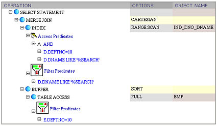
then we see that both Filter and Access predicates can be applied at the same node. Naturally, only d.deptno = 10 conjunct can be used as a start and stop key condition for the index range scan. The dname like '%SEARCH' predicate is then applied as a filter.

Predicates allow us to see artifacts hidden deep under the sql engine hood. For example, consider the following query:

select ename from emp
where ename like 'MIL%'

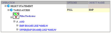
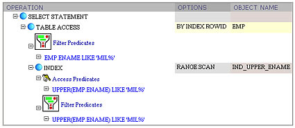
When I saw this plan my natural question was, where did the second conjunct UPPER(ename) like UPPER('MIL%') come from? After a quick investigation, I found that there was a check constraint UPPER(ename) = ename declared upon the emp table. In other words, Oracle leverages check constraints when manipulating query predicates. If we add a function-based index upon UPPER(ename) pseudocolumn, then it would be used, even though the original query doesn't have any function calls within the predicate:

select ename from emp
where ename like 'MIL%'

V$SQL_PLAN_STATISTICS

There is a well known Achilles' heel in SQL optimization: the cost-based plan is as reliable as the cost estimation is. Several factors contribute to inherent difficulty of realistic cost estimation:

1) Complex predicates. Complex predicate expressions include either multiple predicates connected with Boolean connectives, or user-defined functions, domain operators, and subqueries in the individual predicates, or any combination of the above. For example, when estimating selectivity of power(10,sal) + sal > 2000 and sal > 1000 predicate, the first problem we face is estimating selectivity of the power(10,sal) + sal > 2000 conjunct alone. The second problem is an obvious correlation between both conjuncts. In some cases dynamic sampling comes to the rescue, while in the worst case a user would be at the mercy of heuristic - default selectivity.

2) Bind variables. Parse time and execution time in this case are the two conflicting goals. Bind variables were designed to amortize parse time overhead among multiple query executions. It negatively affected the quality of the plans, however, since much less can be inferred about selectivity of a predicate with a bind variable.

3) Data Caching. With caching a simplistic model where the cost is based upon the number of logical IOs is no longer valid: cost model adjustment and caching statistics is necessary.

New dictionary view V$SQL_PLAN_STATISTICS and its sibling V$SQL_PLAN_STATISTICS_ALL (joining the former with V$SQL_PLAN) were introduced in order to help performance analyst to quicker recognize query optimization problems. In my experience, the following two columns are indispensable:

LAST_CR_BUFFER_GETS      NUMBER
LAST_OUTPUT_ROWS         NUMBER

When evaluating the quality of the plan, I measure up the COST against LAST_CR_BUFFER_GETS, and CARDINALITY against LAST_OUTPUT_ROWS. Before V$SQL_PLAN_STATISTICS was introduced it was still possible to know the number of row processed at each plan node (or speaking more accurately - row source) from tkprof output, of course. It also was possible to get cumulative I/O and other statistics for each SQL statement. Statistics table, however, gives itemized report per each plan node, and is, therefore, both more detailed and more convenient.

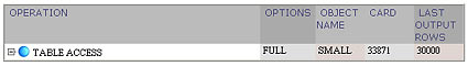
Let's jump to the examples. Our first exercise is fairly trivial: scanning the full table that was not analyzed:

alter session set OPTIMIZER_DYNAMIC_SAMPLING = 0;
select /*+all_rows*/ * from small;

Here, I set OPTIMIZER_DYNAMIC_SAMPLING = 0 because the default setting in Oracle release 2 has been increased to 1, and the hint is used to force CBO mode. The discrepancy between the number of row processed and the estimated cardinality is because there are no statistics on the table. Let's raise sampling level in our experiment:

alter session set OPTIMIZER_DYNAMIC_SAMPLING = 2;
select /*+all_rows*/ * from small;

Now, estimation discrepancy is negligible.

(Sampling levels documentation.)

In our final example, let's explore classic Indexed Nested Loops:

select s1.id,s2.id from small s1, small s2
where s1.id =1 and s1.data=s2.data

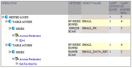
I deliberately made up the example so that each plan node processes one row only. In that case, the execution statistics are quite pronounced. The example starts with a unique index scan of the primary key. Since we have 30000 rows total, then the B-Tree index has three levels, and, therefore, we see exactly three logical I/Os at the plan statistics node. Next, the execution dereferences a pointer from B-Tree leaf to the table row. It's just one more block read. After the row from the driving table is known, the inner block of the Nested Loop can be executed; specifically, index range scan is performed first. Since the result of the range scan is a single B-Tree leaf, the statistics is identical to that of the unique index scan in the outer branch. We therefore have four more block reads. And, finally, the overallexecution I/O is just a sum 4+4=8  of both inner and outer Nested Loops plan branches.

My thanks to Benoit Dageville and Mohamed Zait who implemented those features. I'm also grateful to my colleague Vladimir Barriere, whose comments improved the article.

--

Vadim Tropashko works for Real World Performance group at Oracle Corp. Prior to that he was application programmer and translated The C++ Programming Language by B.Stroustrup, 2nd edition, into Russian. His current interests include SQL Optimization, Constraint Databases, and Computer Algebra Systems.