
Perils and Pitfalls in Partitioning - Part 2
Part 1 | Part 2
This is a continuation of last month's article on partitioning. In case you haven't seen the first part, here it is. Partitioning is a favorite topic for authors, presenters, and for the DBA community in general, but most of the papers on this subject dwell on the basics and fundamental concepts behind partitioning. The inevitable action of most DBAs, after learning the ropes, is to jump into their databases with partitioning in mind. But not so fast. This article describes some the potential problems with partitioning, features with little, or no, documentation that may create unforeseen situations, and how to resolve these. To get the most out of this article, you should already have some basic knowledge about partitioning — this is not a primer.
Multi-Column Partition Keys
Most documentation, articles, books, and so on, talk about a single column as a partitioning key, but how about two or more columns in the partitioning key? It's definitely possible, but in such a case, how should you proceed?
Many people are under the impression that specifying more than one column as partitioning key creates a multi-dimensional partitioned table. For example, if you have a table called “employee range” partitioned on (DEPTNO, ZIPCODE), does that mean that the values of both columns are evaluated when you are deciding about the placement of the row in a partition?
Unfortunately, the answer is - no.
The second column in the partitioning key is used only in some special cases. Both values do not need to be satisfied for an insert to go to a specific partition. The first column is evaluated first; if it satisfies the condition, then the second column is not evaluated. However, if the first column value is borderline satisfactory, the next column is considered.
This is perhaps better explained using an example. Consider the following:
create table ptab1

    col1 number(10),
    col2 number(10),
    col3 varchar2(20)
)
partition by range (col1, col2)
(
partition p1 values less than (101, 101),
partition p2 values less than (201, 201)
)
It is a popular perception that when a row is inserted, if the values of col1 and col2 both are less than 101, then it goes to partition P1; if the values are less than 201, but more than or equal to 101, it goes to partition P2; otherwise, it goes to partition PM. In our example, let's see which partition holds what. Here are all the rows of the table:
select * from ptab1;

COL1             COL2 COL3
---------- ---------- ------
       100        100 rec1
       102        102 rec2
       100        102 rec3
       102        100 rec4
       101        100 rec5
       101        101 rec6
       101        102 rec7
       201        100 rec8
       201        101 rec9
       201        102 rec10
In which partitions do you think the records will be? Let's check the first one:
select * from ptab1 partition (p1);

COL1             COL2 COL3
---------- ---------- ------
       100        100 rec1
       100        102 rec3
       101        100 rec5
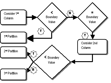
Record rec1 is in partition P1 as expected. But should rec3 be in partition P1? The value of column col1, which is 100, is less than 101 and therefore satisfied. But col2 is 102, and is more than 101, the boundary value of COL2. How does COL2 end up in the P1 partition? The reason is quite simple: P1 is the first partition, it's evaluated for the first column (COL1), the value satisfies it, so the value of column COL2 is not even evaluated. The record goes to P1, even though COL2 is not satisfied.
So, if the second column, col2, is not even considered at all in some cases, where does it come into play and why would you define it? Consider the record REC5, in which the COL1 value is 101, a borderline value of that column in the partitioning key. But in this case, the second column is considered. In this case, COL2 value is 100, less than the boundary value of COL2 in the partitioning key (101); therefore, it goes into the partition P1. Look at the records in partition P2.
select * from ptab1 partition (p2);

COL1             COL2 COL3
---------- ---------- -----
       102        102 rec2
       102        100 rec4
       101        101 rec6
       101        102 rec7
       201        100 rec8
       201        101 rec9
       201        102 rec10
The records rec2, REC4, and REC7 satisfy both columns and are as expected in partition P2. However, for rec6, the col1 value is 101, which is the boundary value for first column of the partitioning key. So, REC6 falls under the special consideration for multi-column partitioning keys. Because the col2 column value of 101 is more than the boundary value of column col2 of partition p1 (101), the rows went to partition P2.
In the same logic, for records REC8, REC9, and REC10, the COL1 value is 201 — right on the boundary for the value of that column in the partitioning key. However, the value of COL2 is less than 201, and the boundary value of that column in P2. Therefore, the rows went to partition P2.
What happens when you insert a row with col1 = 201 and col2 = 201?
That row will go into partition PM, since both columns cannot be outside the bounds. Schematically, the decision to insert into a partition can be explained as in the figure below.
So what happens in the case of list partitioning in Oracle 9i, when there is no concept of a range, so there is no boundary value? Fortunately, list partitioning does not allow multiple columns, so this situation does not arise.
It seemsthat, given the potential confusion about the placement of rows in partitions, it's not worth persuing the use of multi-column partitioning keys. However, in some special cases, it can be very useful. Consider a table called SALES, for instance, with columns SALES_YEAR, SALES_MONTH and SALES_DAY, instead of a single column called SALES_DATE. This is useful in some datawarehouse design implementations to enable dimensions and hierarchies. In such a case, you could use a partitioning key in all three columns to effectively design the partitions.
Potential Pitfall: Be careful while defining multiple columns as partitioning keys. If you must do so, use test cases exactly around the boundary values.
Subpartition Statistics
This is one tricky part of subpartitioning, which is not well documented and clear in the manuals. You must have been using the DBMS_STATS package for quite some time now to collect statistics. To collect statistics for the tables and the sub-objects under them (e.g. , partitions and subpartitions), you should use the function under the package named GATHER_TABLE_STATS. The function has two, little-known parameters that must be set for proper statistics collection.
PARTNAME
This parameter is supposedly set to collect statistics for only the named partition within the table, not for the entire table. However, this is a misconception. PARTNAME can be used to collect the stats for a specific subpartition, too. In order to do that, the name of the subpartition is passed as this parameter.
GRANULARITY
This parameter instructs the package to collect statistics at different levels and to cascade down to other sub-objects. It accepts several values. The default, named DEFAULT, instructs the package to collect global statistics and on the partitions only. The PARTITION value instructs the package to collect stats at the partition level. However, setting these values will not collect stats at the subpartition level; these can be collected by setting the parameter to ALL or SUBPARTITON.
Consider the table created as follows:
create table spart1
(
   col1    number,
   col2    number,
   col3    varchar2(20)
)
partition by range (col1)
subpartition by hash (col2)
subpartitions 4
(
   partition p1 values less than (101),
   partition p2 values less than (201),
   partition p3 values less than (301),
   partition p4 values less than (401),
   partition pm values less than (maxvalue)
)
Analyze the table using the default value of granularity as follows:
exec dbms_stats.gather_table_stats (tabname=>'SPART1')
Note, we have not provided the granularity at all. Since the default value is to collect stats for the partitions only, and not for any of the subpartitions, the stats will not be collected for the subpartitions. This can be verified by issuing:
select partition_name
from user_tab_subpartitions
where last_analyzed is not null;
This command will not return any rows. But let's analyze the other options here. A table can have statistics at the table level only, called GLOBAL statistics. If the partitions of the table are analyzed and the optimizer can derive the global statstics from the individual partitions, then the stats for the table are supposed to be derived globally. Let's examine each option in detail:
exec dbms_stats.gather_table_stats (tabname=>'SPART1', granularity=>'GLOBAL')
This collects stats at the global level only. The following query confirms this.
Select last_analyzed, global_stats
From user_tables where table_name = 'SPART1';
This returns
GLO LAST_ANAL
--- ---------
YES 10-MAR-03
The presence of global stats indicates that the table has been analyzed as a whole, but the optimizer will not know the stats of individual partitions. This can be gathered using:
exec dbms_stats.gather_table_stats (tabname=>'SPART1', granularity=>'PARTITION')
This command sets the stats at the partition level only. In this case, the global stats are not collected on the table, and the query above will return a NO under GLOBAL_STATS. However, the query
select partition_name, last_analyzed
from user_tab_partitions
where last_analyzed is not null;
will retrieve all the partitions. Another variation of the package is shown below.
exec dbms_stats.gather_table_stats (tabname=>'SPART1',
granularity=>'SUBPARTITION')
This collects stats on the subpartition level only, and infers the stats on the partition level; however, it does not collect global stats on the partitions itself.
The last value of the option, ALL, performs all of these — collects partition-level, and subpartition level stats, as well as the global stats on the subpartition, partition, and table.
Thus, the default value for the GRANULARITY parameter in the stats gathering function does not collect stats on subpartitions; you must set it to either SUBPARTITION or ALL to gather stats.
In summary, here are the details about setting granularity and collecting statistics:
| GRANULARITY | Table Global | Partition Global | Partition Statistics | Subpartition Statistics |
| GLOBAL | YES | NO | NO | NO |
| PARTITION | NO | YES | YES | NO |
| DEFAULT | YES | YES | YES | NO |
| SUBPARTITION | NO | NO | YES | YES |
| ALL | YES | YES | YES | YES |
Another interesting concept that is not documented clearly is the option to analyze subpartitions only. This can be done using:
exec dbms_stats.gather_table_stats (tabname=>'SPART1', PART_NAME=>'P1_SYS123')
This will collect subpartition-level stats on subpartition P1_SYS123 only.
Rule Based Optimizer
Can you use partitioning with Rule Based Optimizer (RBO)? The answer is, of course you can. However, when partitioning was introduced, RBO was considered legacy, and Oracle decided to gradually phase out support for it. This led to a general stop in development of RBO, so today, RBO is not set up to exploit several exciting developments, partitioning included. Therefore, to get the full advantage of partitioning (partition pruning, partition-wise joins, and so on), you must use the Cost Based Optimizer (CBO). If you use the RBO, and a table in the query is partitioned, Oracle kicks in the CBO while optimizing it. But because the statistics are not present, the CBO makes up the statistics, and this could lead to severely expensive optimization plans and extremely poor performance.
So, although you can, you shouldn't use partitioning when using the RBO.
Coalesce vs. Merge
These two potentially confusing statements serve the same purpose — reducing the number of partitions – and are applicable in different schemes. In a range- or list-partitioned table, the partition boundaries are clearly defined, and the rows in a partition satisfy some condition dependent on the boundary values. ALTER TABLE … MERGE PARTITION joins the two adjacent partitions and sets the boundary values appropriately.
Consider the example of a table PART that is partitioned by range into four different partitions named P1, P2, P3, and P4. To merge partitions P3 and P4 to make a partition called P34, issue the following statement:
ALTER TABLE PART MERGE PARTITIONS P3, P4 INTO PARTITION P34;
However, in hash-partitioned tables, there are no boundary values, and the rows are not decided as candidates for the partitions based on some kind of defined range. So, a merge will not be able to identify and set specific boundaries. You should use a new clause called COALESCE to achieve this objective:
ALTER TABLE PART COALESCE;
In COALESCE, a specific partition, usually the last one, is identified for elimination. All the rows in that partition are supposed to be equally distributed over the remaining partitions and the partition is dropped. In practice, however, the rows are merged with the adjacent partition.
Since this reduces the number of partitions by one, the total number is not a power of two any more, making the distribution of rows in all partitions unequal. To avoid this problem, issue the COALESCE one more time to make the partitions evenly loaded.
In summary, MERGE is for range and list partitioning when the values are clearly identified for boundary values, and COALESCE is for hash partitions, to reduce the number of partitions.
Other Questions
What about Rebuild Partition and Global Indexes?
Oracle9iR2 now offers fast split partitioning. Typically, during a split operation, Oracle creates two new partitions and then redistributes the rows from the source partition to the new partitions. This is a very expensive operation from the resource consumption point of view. In addition, local index partitions become unusable.
With fast split partitioning, if all the rows will exist in the same partition after the partition split, Oracle simply reuses the old partition and creates an empty partition. Thus, a split action becomes more like a complete operation that just creating a new partition.
Global indexes become unusable when a partition is rebuilt. However, in 9i, a new clause updates the global indexes as well.
ALTER TABLE PTAB DROP PARTITION P2 UPDATE GLOBAL INDEXES;
While using partitioning, should you use bind variables?
This is an interesting question. As we all know, use of bind variables eliminates the need to parse the cursors and makes it easier to reuse the cursors.
In case of partitions, however, using bind variables poses a problematic situation. Partition elimination and joins can occur only if the optimizer knows the filtering predicate in advance. The value of bind variables are not known until it's time to execute, making the process of partition elimination or joins impossible. Therefore, to take advantage of these options, you should not use bind variables.
In Oracle 9i, the first parse of the statement, called hard parse, peeks into the value of the bind variable, and can effect these optimization options. But this occurs only with the hard parse; subsequent parses still go around the bind variable values.
How many partitions can be defined on a table?
Oracle uses a two-byte field to store the number of segments (partitions or subpartitions), which enables 2^16 or 65536 spaces. The Oracle code, therefore, allows one fewer than this number — 65535. Note that this is a limit set by Oracle software code; an actual limit may be lower.
Remember, every time a query is parsed on a partitioned object, the metadata (i.e., how many partitions, and so on) is loaded into the cursor cache in SGA, meaning the SGA should be large enough to handle a table with several partitions.
--
Arup Nanda has been an Oracle DBA for 10 years. He is the founder of Proligence, Inc., a New York-area company that provides specialized Oracle database services. He is also an editor of SELECT, the journal of the International Oracle User Group. He has written Oracle technical articles in several national and international journals like SELECT, Oracle Scene, SQLUPDATE and presented in several conferences like Oracle Technology Symposium, Atlantic Oracle Training Conference, IOUG Live! among others. Send feedback to Arup about this article at arup@proligence.com. Based on the feedback, an updated copy of this article can be found at www.proligence.com.
Contributors : Arup Nanda
Last modified 2006-01-05 10:39 AM
If you use literals, then Oracle can work out which partitions to eliminate at parse time (here is an extract from a 10046 trace)
SELECT COUNT(*) FROM SPART1 WHERE COL1 = 42
END OF STMT
STAT #3 id=1 cnt=1 pid=0 pos=1 obj=0 op='SORT AGGREGATE '
STAT #3 id=2 cnt=1 pid=1 pos=1 obj=86954 op='TABLE ACCESS FULL SPART1 PARTITION: 1 1 '
IF you use bind variables, the Oracle know it should be able to eliminate partitions but it doesn't know which ones until execution. But it will eliminate partitions.
SELECT COUNT(*) FROM SPART1 WHERE COL1 = :B1
END OF STMT
STAT #2 id=1 cnt=1 pid=0 pos=1 obj=0 op='SORT AGGREGATE '
STAT #2 id=2 cnt=1 pid=1 pos=1 obj=0 op='PARTITION RANGE SINGLE PARTITION: KEY KEY '
STAT #2 id=3 cnt=1 pid=2 pos=1 obj=86954 op='TABLE ACCESS FULL SPART1 PARTITION: KEY KEY '