
Trees in SQL: Nested Sets and Materialized Path
Relational databases are universally conceived of as an advance over their predecessors network and hierarchical models. Superior in every querying respect, they turned out to be surprisingly incomplete when modeling transitive dependencies. Almost every couple of months a question about how to model a tree in the database pops up at the comp.database.theory newsgroup. In this article I'll investigate two out of four well known approaches to accomplishing this and show a connection between them. We'll discover a new method that could be considered as a "mix-in" between materialized path and nested sets.
Adjacency List
Tree structure is a special case of Directed Acyclic Graph (DAG). One way to represent DAG structure is:
create table emp (
   ename   varchar2(100),
   mgrname varchar2(100)
);
Each record of the emp table identified by ename is referring to its parent mgrname. For example, if JONES reports to KING, then the emp table contains <ename='JONES', mgrname='KING'> record. Suppose, the emp table also includes <ename='SCOTT', mgrname='JONES'>. Then, if the emp table doesn't contain the <ename='SCOTT', mgrname='KING'> record, and the same is true for every pair of adjoined records, then it is called adjacency list. If the opposite is true, then the emp table is a transitively closed relation.
A typical hierarchical query would ask if SCOTT indirectly reports to KING. Since we don't know the number of levels between the two, we can't tell how many times to selfjoin emp, so that the task can't be solved in traditional SQL. If transitive closure tcemp of the emp table is known, then the query is trivial:
select 'TRUE' from tcemp
where ename = 'SCOTT' and mgrname = 'KING'
The ease of querying comes at the expense of transitive closure maintenance.
Alternatively, hierarchical queries can be answered with SQL extensions: either SQL3/DB2 recursive query
with tcemp as (
    select ename,mgrname from tcemp
  union
    select tcemp.ename,emp.mgrname from tcemp,emp
    where tcemp.mgrname = emp.ename
) select 'TRUE' from tcemp
where ename = 'SCOTT' and mgrname = 'KING';
that calculates tcemp as an intermediate relation, or Oracle proprietary connect-by syntax
select 'TRUE' from (
  select ename from emp
  connect by prior mgrname = ename
  start with ename = 'SCOTT'
) where ename = 'KING';
in which the inner query "chases the pointers" from the SCOTT node to the root of the tree, and then the outer query checks whether the KING node is on the path.
Adjacency list is arguably the most intuitive tree model. Our main focus, however, would be the following two methods.
Materialized Path
In this approach each record stores the whole path to the root. In our previous example, lets assume that KING is a root node. Then, the record with ename = 'SCOTT' is connected to the root via the path SCOTT->JONES->KING. Modern databases allow representing a list of nodes as a single value, but since materialized path has been invented long before then, the convention stuck to plain character string of nodes concatenated with some separator; most often '.' or '/index.html'. In the latter case, an analogy to pathnames in UNIX file system is especially pronounced.
In more compact variation of the method, we use sibling numerators instead of node's primary keys within the path string. Extending our example:
| ENAME | PATH |
| KING | 1 |
| JONES | 1.1 |
| SCOTT | 1.1.1 |
| ADAMS | 1.1.1.1 |
| FORD | 1.1.2 |
| SMITH | 1.1.2.1 |
| BLAKE | 1.2 |
| ALLEN | 1.2.1 |
| WARD | 1.2.2 |
| CLARK | 1.3 |
| MILLER | 1.3.1 |
Path 1.1.2 indicates that FORD is the second child of the parent JONES.
Let's write some queries.
1. An employee FORD and chain of his supervisors:
select e1.ename from emp e1, emp e2
where e2.path like e1.path || '%'
and e2.name = 'FORD'
2. An employee JONES and all his (indirect) subordinates:
select e1.ename from emp e1, emp e2
where e1.path like e2.path || '%'
and e2.name = 'JONES'
Although both queries look symmetrical, there is a fundamental difference in their respective performances. If a subtree of subordinates is small compared to the size of the whole hierarchy, then the execution where database fetches e2 record by the name primary key, and then performs a range scan of e1.path, which is guaranteed to be quick.
On the other hand, the "supervisors" query is roughly equivalent to
select e1.ename from emp e1, emp e2
where e2.path > e1.path and e2.path < e1.path || 'Z'
and e2.name = 'FORD'
Or, noticing that we essentially know e2.path, it can further be reduced to
select e1.ename from emp e1
where e2path > e1.path and e2path < e1.path || 'Z'
Here, it is clear that indexing on path doesn't work (except for "accidental" cases in which e2path happens to be near the domain boundary, so that predicate e2path > e1.path is selective).
The obvious solution is that we don't have to refer to the database to figure out all the supervisor paths! For example, supervisors of 1.1.2 are 1.1 and 1. A simple recursive string parsing function can extract those paths, and then the supervisor names can be answered by
select e1.ename from emp where e1.path in ('1.1','1')
which should be executed as a fast concatenated plan.
Nested Sets
Both the materialized path and Joe Celko's nested sets provide the capability to answer hierarchical queries with standard SQL syntax. In both models, the global position of the node in the hierarchy is "encoded" as opposed to an adjacency list of which each link is a local connection between immediate neighbors only. Similar to materialized path, the nested sets model suffers from supervisors query performance problem:
select p2.emp from Personnel p1, Personnel p2
where p1.lft between p2.lft and p2.rgt
and p1.emp = 'Chuck'
(Note: This query is borrowed from the previously cited Celko article). Here, the problem is even more explicit than in the case of a materialized path: we need to find all the intervals that cover a given point. This problem is known to be difficult. Although there are specialized indexing schemes like R-Tree, none of them is as universally accepted as B-Tree. For example, if the supervisor's path contains just 10 nodes and the size of the whole tree is 1000000, none of indexing techniques could provide 1000000/10=100000 times performance increase. (Such a performance improvement factor is typically associated with index range scan in a similar, very selective, data volume condition.)
Unlike a materialized path, the trick by which we computed all the nodes without querying the database doesn't work for nested sets.
Another — more fundamental — disadvantage of nested sets is that nested sets coding is volatile. If we insert a node into the middle of the hierarchy, all the intervals with the boundaries above the insertion point have to be recomputed. In other words, when we insert a record into the database, roughly half of the other records need to be updated. This is why the nested sets model received only limited acceptance for static hierarchies.
Nested sets are intervals of integers. In an attempt to make the nested sets model more tolerant to insertions, Celko suggested we give up the property that each node always has (rgt-lft+1)/2 children. In my opinion, this is a half-step towards a solution: any gap in a nested set model with large gaps and spreads in the numbering still could be covered with intervals leaving no space for adding more children, if those intervals are allowed to have boundaries at discrete points (i.e., integers) only. One needs to use a dense domain like rational, or real numbers instead.
Nested Intervals
Nested intervals generalize nested sets. A node [clft, crgt] is an (indirect) descendant of [plft, prgt] if:
plft <= clft and crgt >= prgt
The domain for interval boundaries is not limited by integers anymore: we admit rational or even real numbers, if necessary. Now, with a reasonable policy, adding a child node is never a problem. One example of such a policy would be finding an unoccupied segment [lft1, rgt1] within a parent interval [plft, prgt] and inserting a child node [(2*lft1+rgt1)/3, (rgt1+2*lft)/3]:
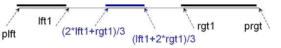
After insertion, we still have two more unoccupied segments [lft1,(2*lft1+rgt1)/3] and [(rgt1+2*lft)/3,rgt1] to add more children to the parent node.
We are going to amend this naive policy in the following sections.
Partial Order
Let's look at two-dimensional picture of nested intervals. Let's assume that rgt is a horizontal axis x, and lft is a vertical one - y. Then, the nested intervals tree looks like this:
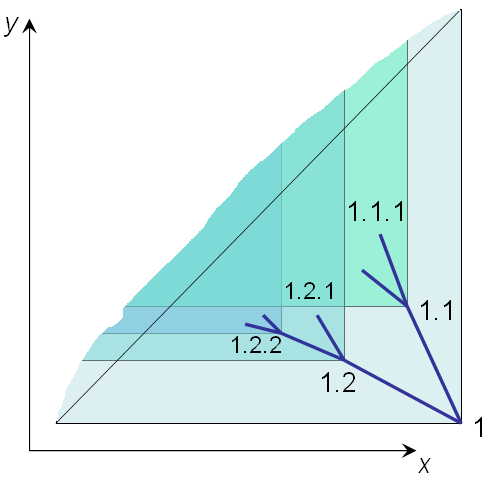
Each node [lft, rgt] has its descendants bounded within the two-dimensional cone y >= lft & x <= rgt. Since the right interval boundary is always less than the left one, none of the nodes are allowed above the diagonal y = x.
The other way to look at this picture is to notice that a child node is a descendant of the parent node whenever a set of all points defined by the child cone y >= clft & x <= crgt is a subset of the parent cone y >= plft & x <= prgt. A subset relationship between the cones on the plane is a partial order.
Now that we know the two constraints to which tree nodes conform, I'll describe exactly how to place them at the xy plane.
The Mapping
Tree root choice is completely arbitrary: we'll assume the interval [0,1] to be the root node. In our geometrical interpretation, all the tree nodes belong to the lower triangle of the unit square at the xy plane.
We'll describe further details of the mapping by induction. For each node of the tree, let's first define two important points at the xy plane. The depth-first convergence point is an intersection between the diagonal and the vertical line through the node. For example, the depth-first convergence point for <x=1,y=1/2> is <x=1,y=1>. The breadth-first convergence point is an intersection between the diagonal and the horizontal line through the point. For example, the breadth-first convergence point for <x=1,y=1/2> is <x=1/2,y=1/2>.
Now, for each parent node, we define the position of the first child as a midpoint halfway between the parent point and depth-first convergence point. Then, each sibling is defined as a midpoint halfway between the previous sibling point and breadth-first convergence point:
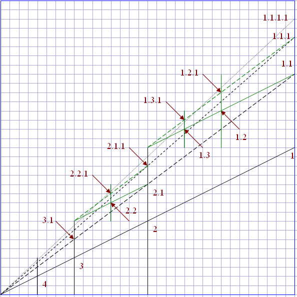
For example, node 2.1 is positioned at x=1/2, y=3/8.
Now that the mapping is defined, it is clear which dense domain we are using: it's not rationals, and not reals either, but binary fractions (although, the former two would suffice, of course).
Interestingly, the descendant subtree for the parent node "1.2" is a scaled down replica of the subtree at node "1.1." Similarly, a subtree at node 1.1 is a scaled down replica of the tree at node "1." A structure with self-similarities is called a fractal.
Normalization
Next, we notice that x and y are not completely independent. We can tell what are both x and y if we know their sum. Given the numerator and denominator of the rational number representing the sum of the node coordinates, we can calculate x and y coordinates back as:
function x_numer( numer integer, denom integer )
RETURN integer IS
ret_num integer;
ret_den integer;
BEGIN
ret_num := numer+1;
ret_den := denom*2;
while floor(ret_num/2b = ret_num/2 loop
ret_num := ret_num/2;
ret_den := ret_den/2;
end loop;
RETURN ret_num;
END;function x_denom( numer integer, denom integer )
...
RETURN ret_den;
END;
in which function x_denom body differs from x_numer in the return variable only. Informally, numer+1 increment would move the ret_num/ret_den point vertically up to the diagonal, and then x coordinate is half of the value, so we just multiplied the denominator by two. Next, we reduce both numerator and denominator by the common power of two.
Naturally, y coordinate is defined as a complement to the sum:
function y_numer( numer integer, denom integer )
RETURN integer IS
num integer;
den integer;
BEGIN
num := x_numer(numer, denom);
den := x_denom(numer, denom);
while den < denom loop
num := num*2;
den := den*2;
end loop;
num := numer - num;
while floor(num/2) = num/2 loop
num := num/2;
den := den/2;
end loop;
RETURN num;
END;function y_denom( numer integer, denom integer )
...
RETURN den;
END;
Now, the test (where 39/32 is the node 1.3.1):
select x_numer(39,32)||'/index.html'||x_denom(39,32),
y_numer(39,32)||'/index.html'||y_denom(39,32) from dual

5/8     19/32

select 5/8+19/32, 39/32 from dual

1.21875 1.21875
I don't use a floating point to represent rational numbers, and wrote all the functions with integer arithmetics instead. To put it bluntly, the floating point number concept in general, and the IEEE standard in particular, is useful for rendering 3D-game graphics only. In the last test, however, we used a floating point just to verify that 5/8 and 19/32, returned by the previous query, do indeed add to 39/32.
We'll store two integer numbers — numerator and denominator of the sum of the coordinates x and y — as an encoded node path. Incidentally, Celko's nested sets use two integers as well. Unlike nested sets, our mapping is stable: each node has a predefined placement at the xy plane, so that the queries involving node position in the hierarchy could be answered without reference to the database. In this respect, our hierarchy model is essentially a materialized path encoded as a rational number.
Finding Parent Encoding and Sibling Number
Given a child node with numer/denom encoding, we find the node's parent like this:
function parent_numer( numer integer, denom integer )
RETURN integer IS
ret_num integer;
ret_den integer;
BEGIN
if numer=3 then
return NULL;
end if;
ret_num := (numer-1)/2;
ret_den := denom/2;
while floor((ret_num-1)/4) = (ret_num-1)/4 loop
ret_num := (ret_num+1)/2;
ret_den := ret_den/2;
end loop;
RETURN ret_num;
END;function parent_denom( numer integer, denom integer )
...
RETURN ret_den;
END;
The idea behind the algorithm is the following: If the node is on the very top level — and all these nodes have a numerator equal to 3 — then the node has no parent. Otherwise, we must move vertically down the xy plane at a distance equal to the distance from the depth-first convergence point. If the node happens to be the first child, then that is the answer. Otherwise, we must move horizontally at a distance equal to the distance from the breadth-first convergence point until we meet the parent node.
Here is the test of the method (in which 27/32 is the node 2.1.2, while 7/8 is 2.1):
select parent_numer(27,32)||'/index.html'||parent_denom(27,32) from dual7/8
In the previous method, counting the steps when navigating horizontally would give the sibling number:
function sibling_number( numer integer, denom integer )
RETURN integer IS
   ret_num integer;
   ret_den integer;
   ret integer;
BEGIN
   if numer=3 then
      return NULL;
   end if;
   ret_num := (numer-1)/2;
   ret_den := denom/2;
   ret     := 1;
   while floor((ret_num-1)/4) = (ret_num-1)/4 loop
      if ret_num=1 and ret_den=1 then
         return ret;
      end if;
      ret_num := (ret_num+1)/2;
      ret_den := ret_den/2;
      ret     := ret+1;
   end loop;
   RETURN ret;
END;
For a node at the very first level a special stop condition, ret_num=1 and ret_den=1 is needed.
The test:
select sibling_number(7,8) from dual1
Calculating Materialized Path and Distance between nodes
Strictly speaking, we don't have to use a materialized path, since our encoding is an alternative. On the other hand, a materialized path provides a much more intuitive visualization of the node position in the hierarchy, so that we can use the materialized path for input and output of the data if we provide the mapping to our model.
Implementation is a simple application of the methods from the previous section. We print the sibling number, jump to the parent, then repeat the above two steps until we reach the root:
function path( numer integer, denom integer )
RETURN varchar2 IS
BEGIN
   if numer is NULL then
      return '';
   end if;
   RETURN path(parent_numer(numer, denom),
               parent_denom(numer, denom))
     || '.' || sibling_number(numer, denom);
END;

select path(15,16) from dual

.2.1.1
Now we are ready to write the main query: given the 2 nodes, P and C, when P is the parent of C? A more general query would return the number of levels between P and C if C is reachable from P, and some exception indicator; otherwise:
function distance( num1 integer, den1 integer,
                   num2 integer, den2 integer )
RETURN integer IS
BEGIN
   if num1 is NULL then
      return -999999;
   end if;
   if num1=num2 and den1=den2 then
      return 0;
   end if;
   RETURN 1+distance(parent_numer(num1, den1),
                     parent_denom(num1, den1),
            num2,den2);
END;

select distance(27,32,3,4) from dual

2
Negative numbers are interpreted as exceptions. If the num1/den1 node is not reachable from num2/den2, then the navigation converges to the root, and level(num1/den1)-999999 would be returned (readers are advised to find a less clumsy solution).
The alternative way to answer whether two nodes are connected is by simply calculating the x and y coordinates, and checking if the parent interval encloses the child. Although none of the methods refer to disk, checking whether the partial order exists between the points seems much less expensive! On the other hand, it is just a computer architecture artifact that comparing two integers is an atomic operation. More thorough implementation of the method would involve a domain of integers with a unlimited range (those kinds of numbers are supported by computer algebra systems), so that a comparison operation would be iterative as well.
Our system wouldn't be complete without a function inverse to the path, which returns a node's numer/denom value once the path is provided. Let's introduce two auxiliary functions, first:
function child_numer
( num integer, den integer, child integer )
RETURN integer IS
BEGIN
   RETURN num*power(2, child)+3-power(2, child);
END;

function child_denom
( num integer, den integer, child integer )
RETURN integer IS
BEGIN
   RETURN den*power(2, child);
END;

select child_numer(3,2,3) || '/index.html' ||
       child_denom(3,2,3) from dual

19/16
For example, the third child of the node 1 (encoded as 3/2) is the node 1.3 (encoded as 19/16).
The path encoding function is:
function path_numer( path varchar2 )
RETURN integer IS
   num integer;
   den integer;
   postfix varchar2(1000);
   sibling varchar2(100);
BEGIN
   num := 1;
   den := 1;
   postfix := '.' || path || '.';

   while length(postfix) > 1 loop
      sibling := substr(postfix, 2,
                        instr(postfix,'.',2)-2);
      postfix := substr(postfix,
                        instr(postfix,'.',2),
                              length(postfix)
                             -instr(postfix,'.',2)+1);
      num := child_numer(num,den,to_number(sibling));
      den := child_denom(num,den,to_number(sibling));
end loop;

RETURN num;
END;

function path_denom( path varchar2 )
...
RETURN den;
END;

select path_numer('2.1.3') || '/index.html' ||
       path_denom('2.1.3') from dual
51/64
The Final Test
Now that the infrastructure is completed, we can test it. Let's create the hierarchy
create table emps (
name varchar2(30),
numer integer,
denom integer
)alter table emps
ADD CONSTRAINT uk_name UNIQUE (name) USING INDEX
(CREATE UNIQUE INDEX name_idx on emps(name))
ADD CONSTRAINT UK_node
UNIQUE (numer, denom) USING INDEX
(CREATE UNIQUE INDEX node_idx on emps(numer, denom))
and fill it with some data:
insert into emps values ('KING',
      path_numer('1'),path_denom('1'));
insert into emps values ('JONES',
      path_numer('1.1'),path_denom('1.1'));
insert into emps values ('SCOTT',
      path_numer('1.1.1'),path_denom('1.1.1'));
insert into emps values ('ADAMS',
      path_numer('1.1.1.1'),path_denom('1.1.1.1'));
insert into emps values ('FORD',
      path_numer('1.1.2'),path_denom('1.1.2'));
insert into emps values ('SMITH',
      path_numer('1.1.2.1'),path_denom('1.1.2.1'));
insert into emps values ('BLAKE',
      path_numer('1.2'),path_denom('1.2'));
insert into emps values ('ALLEN',
      path_numer('1.2.1'),path_denom('1.2.1'));
insert into emps values ('WARD',
      path_numer('1.2.2'),path_denom('1.2.2'));
insert into emps values ('MARTIN',
      path_numer('1.2.3'),path_denom('1.2.3'));
insert into emps values ('TURNER',
      path_numer('1.2.4'),path_denom('1.2.4'));
insert into emps values ('CLARK',
      path_numer('1.3'),path_denom('1.3'));
insert into emps values ('MILLER',
      path_numer('1.3.1'),path_denom('1.3.1'));
commit;
All the functions written in the previous sections are conveniently combined in a single view:
create or replace
view hierarchy as
  select name, numer, denom,
         y_numer(numer,denom) numer_left,
         y_denom(numer,denom) denom_left,
         x_numer(numer,denom) numer_right,
         x_denom(numer,denom) denom_right,
         path (numer,denom) path,
         distance(numer,denom,3,2) depth
  from emps
And, finally, we can create the hierarchical reports.
- Depth-first enumeration, ordering by left interval boundary
select lpad(' ',3*depth)||name
from hierarchy order by numer_left/denom_left
LPAD('',3*DEPTH)||NAME
-----------------------------------------------
KING
   CLARK
      MILLER
   BLAKE
      TURNER
      MARTIN
      WARD
      ALLEN
   JONES
      FORD
         SMITH
      SCOTT
         ADAMS
- Depth-first enumeration, ordering by right interval boundary
select lpad(' ',3*depth)||name
from hierarchy order by numer_right/denom_right desc
LPAD('',3*DEPTH)||NAME
-----------------------------------------------------
KING
   JONES
      SCOTT
         ADAMS
      FORD
         SMITH
   BLAKE
      ALLEN
      WARD
      MARTIN
      TURNER
   CLARK
      MILLER
- Depth-first enumeration, ordering by path (output identical to #2)
select lpad(' ',3*depth)||name
from hierarchy order by path
LPAD('',3*DEPTH)||NAME
-----------------------------------------------------
KING
   JONES
      SCOTT
         ADAMS
      FORD
         SMITH
   BLAKE
      ALLEN
      WARD
      MARTIN
      TURNER
   CLARK
      MILLER
- All the descendants of JONES, excluding himself:
select h1.name from hierarchy h1, hierarchy h2
where h2.name = 'JONES'
and distance(h1.numer, h1.denom,
h2.numer, h2.denom)>0;NAME
------------------------------
SCOTT
ADAMS
FORD
SMITH
- All the ancestors of FORD, excluding himself:
select h2.name from hierarchy h1, hierarchy h2
where h1.name = 'FORD'
and distance(h1.numer, h1.denom,
h2.numer, h2.denom)>0;NAME
------------------------------
KING
JONES
--
Vadim Tropashko works for Real World Performance group at Oracle Corp. In prior life he was application programmer and translated "The C++ Programming Language" by B.Stroustrup, 2nd edition into Russian. His current interests include SQL Optimization, Constraint Databases, and Computer Algebra Systems.
Contributors : Vadim Tropashko
Last modified 2005-04-13 02:49 PM
 ints too small
0.01001011
and the path is: x2xx3x21
This implies the sum of the node numbers equals the number of binary digits required to express the numerator. Clearly you are going to run out if you use a normal 32 or 64 bit int. In this sense it has the same problems as chelko's proposal.
For run, I analysed our portfolio hierarchy. We would need 115 bits to represent the numerator for 2344 portfolios.
function sibling_number( numer integer, denom integer )
RETURN integer IS
ret_num integer;
ret_den integer;
ret integer;
BEGIN
if numer=3 then
return NULL;
end if;
....
RETURN ret;
END;
[/quote]
Is this behaviour really correct? What if we have numer=3 and denom=4. I'd rather expect sibling_number(numer, denom) to return integer 2, but never NULL.
( I realize that the article doesn't focus on details of impementation, but nonetheless... )
Replies to this comment