Part 1  |  Part 2  |  Part 3

In an earlier article, I described the basic functionality of bitmap indexes, describing in particular their relevance to DSS types of system where data updates were rare, and indexes could be dropped and rebuilt for data loads. In this article we move onwards to one of the more advanced features of bitmap indexes, namely the bitmap star transformation that first appeared in later versions of Oracle 7.

In an earlier article I demonstrated the extraordinary effectiveness of bitmap indexes when addressing queries of the type shown in figure 1.

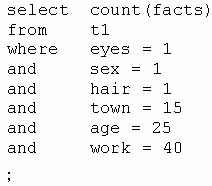Figure 1: A query designed for Bitmap Indexes.

If facts was a very large table with single column bitmap indexes on each of the columns eyes, sex, hair, town, age, and work, then Oracle could use normal costing techniques to decide that a combination of some (not necessarily all) of these indexes could be used through the mechanism of the bitmap AND to answer the query.

Of course, I pointed out that while such bitmap indexes could be used very effectively for queries, there were serious performance penalties if the indexes were in place when data maintenance was going on. These penalties essentially required you to consider dropping and rebuilding your bitmap indexes as part of your data maintenance procedures.

However, there is a rather more significant weakness in this example that means it is not really a good example of genuine end-user requirements. It is often the case that the actual values we wish to use to query the data are not stored on the main data table. In real systems, they tend to be stored in related dimension tables.

For example, we might have a table of Towns in which code 15 represents Birmingham. The end-user could quite reasonably expect to query the facts table in terms of Birmingham rather than using a meaningless code number. Of course, the query might even be based on a secondary reference table States(where the column state_id is a foreign key in Towns) if we were interested in all the towns in Alabama.

This issue is addressed by the Bitmap Star Transformation, a mechanism introduced in Oracle 7 although its use is still not the default behavior, even in Oracle 9.2, in which the two relevant parameters,

     _always_star_transformation

     star_transformation_enabled

still have the default value of FALSE. (Note: the star transformation is not the same as the star query that was introduced in earlier versions of Oracle 7 and was dependent on massive, multi-column b-tree indexes.)

A new feature of Oracle 9.2, the bitmap join index, may also be of benefit in such queries, but the jury is still out on that one, and I plan to describe that mechanism and comment on it in a later feature.

The Bitmap Star Transformation

What is a Bitmap Star Transformation, how do you implement it, and how do you know that it is working?

The main components are a large fact table and a surrounding collection of dimension tables. A row in the fact table consists of a number of useful data elements, and a set of identifiers - typically short codes. Each identifying column has a bitmap index created over it.

An identifying column on the fact table corresponds to one of the dimension tables, and the short codes that appear in that column must be selected from the (declared) primary key of that table. Figure 2 shows an extract from a suitable set of table definitions:

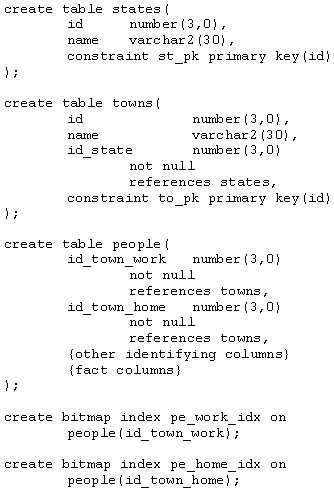
Figure 2: Part of a Star (snowflake) Schema.

In this example, we have a people table as the central fact table, and a towns table, which is actually used twice as a dimension table. I have also included a states table representing the relationship that each town is in a state. This is to illustrate the fact that Oracle can actually recognize a "snowflake" schema. (Refer to figure 3.)

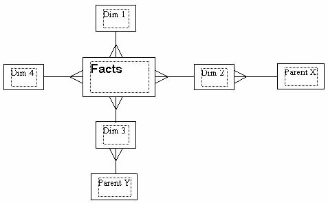Figure 3: Simple Snowflake Schema.

You will note that I have declared foreign key referential integrity between the people table and the towns table. There are two points to bear in mind here. First, that the presence of the bitmap index is not sufficient to avoid the share lock problem that shows up if you update or delete a parent id - an index created for this purpose has to be a b-tree index. (Of course, in a DSS database, such updates are not likely to be a significant issue.) Second, for reasons that will be discussed in future articles on materialized views and partitioned tables, such foreign key constraints in DSS databases are quite likely to be declared as disabled, not validated, and rely.

Having created the tables, loaded them with suitable data, and then enabled the feature by issuing:

    alter session set

        star_transformation_enabled =


            true;

we can start to examine the execution plans for queries such as those in figure 4.

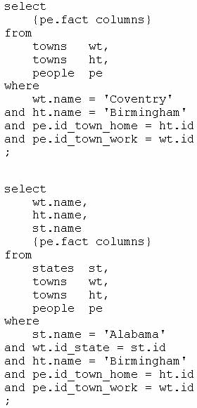Figure 4: Sample Queries.

There are several variations in the gross structure of the execution plan that depend on whether we are using a simple star transformation, or a more complex query. The most important point to note in the execution plan, though, is the presence of lines like those in figure 5 (which almost a complete plan for the first query in figure 4).

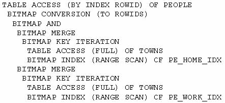
Figure 5: Baseline Execution Plan.

Reading the plan recursively from top to bottom, we see that the path is:

• Examine the towns table for towns called "Birmingham," and find the primary key of each such town. For each Birmingham primary key in turn, scan the bitmap index pe_home_idx for the relevant section. Merge the resulting sections into a single large bitmap for the possible target rows of the people table.
• Repeat the process for "Coventry" and the PE_work_idx index to produce a second large bitmap.
  
  (For more complex schemas, the above step will be repeated, perhaps for every dimension specified in the query, to produced one bitmap per dimension.)
• AND the two bitmaps together to produce a single bitmap identifying all people rows that match both conditions.
• Convert the resulting bitmap into a list of rowids, and fetch the rows from the table.

Notice how this stage of the operation, targets and returns the smallest possible set of people rows with the minimum expenditure of resources. Dimension tables are usually relatively small, so the cost of finding their primary keys is low; the bitmap indexes on the people table are relatively small, so scanning them for each towns key value is quite cheap, and the bitmap AND operation is very efficient.

Remember — in many cases, the most expensive action in a query is the work of collecting the actual rows from the largest table(s). A mechanism like the bitmap star transformation that manages to identify exactly the bare minimum number of rows from the fact table, with no subsequent discards, can give you a terrific performance gain.

Once we have established that the critical section of the plan is appearing, we can worry about the extra work that may have to be done.

For example, in the second query in figure 4, we want columns from the towns table(s), as well as moving out one extra layer to get data from the states table. Because we have started with a star transformation to identify the critical people rows, we should now join this 'intermediate result set' back to the dimension tables with a minimum of extra work.

So the questions we need to ask are - do we still see the same pattern of AND'ed bitmaps in the plan, and what can we see that shows us how the extra columns handled.

To answer the first question, the inner part of the plan now looks like figure 6. The same basic structure of the star transformation is clearly visible even though one (highlighted) part of it now includes a join to the states table. This is the critical section of code that ensures we locate the minimum set of people rows that are relevant, and use the minimum resources to get them.

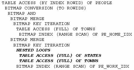Figure 6: Core of Extended Plan.

What about the rest of the data, though — how does Oracle retrieve the extra columns that have not been required so far? The full plan — simplified by replacing the section shown in figure 6 by a single line — is likely to be something similar to the one shown figure 7:

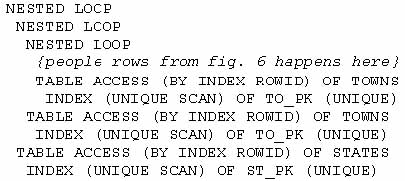
Figure 7: Revisiting the Fact Tables.

The sub-plan shown above simply says — for each row found in the people table get the home town using the primary key, then get the work town by primary key, then get the state by primary key.

In effect, the query has been rewritten internally in the form shown in figure 8, where we can more easily see the first half of the where clause becoming the driving bitmap access clause, and the second half of the clause being used to join back to the dimension tables.

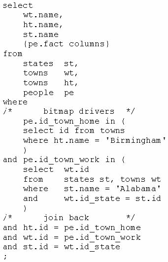Figure 8: Notional Internal rewrite.

As ever, there are numerous variations on a theme.

• Oracle may be able to restructure b-tree information into bitmap form in memory, so extra conversion steps may appear in the plan.
• The bitmap star transformation can be applied to partitioned tables, so extra steps relating to partitioning may appear.
• The path can execute in parallel, introducing extra levels of messy parallel distribution elements in the plan.
• The join back of the dimension tables could be implemented as a series of hash joins, or sort merge joins instead of nested loop joins.

Warnings

One important detail to watch out for is that the bitmap star transformation is available only to the Cost Based Optimizer (after all, the Rule Based Optimizer doesn't even recognize bitmap indexes). So, if you fail to generate statistics of a suitable quality, the optimizer may very easily switch into an alternative plan — typically a very expensive, multistage hash join mechanism.

Of course, there is also the critical detail that you can't do the bitmap star transformation without using bitmap indexes, and these are only available with the Enterprise Edition.

Also, be aware that under newer versions of Oracle, a recursive temporary table mechanism may be use to handle the dimension tables. At present tkprof, autotrace, and v$sql_plan have no method of showing you what is going on behind the scenes, so you will need the latest SQL code for reporting the results of an explain plan.

For example, the second query of figure 4 might produce an autotrace plan including lines like those in figure 9:

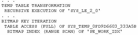Figure 9: Temp Table Transformation *extract).

You may be able to guess this has something to do with the join between (work) towns and states because those two tables will have vanished from the plan. But without the aid of the latest SQL for reporting the results of explain plan, you won't be able to see that the recursive step is creating and populating a temporary table using SQL, such as:

    INSERT INTO

    SYS.SYS_TEMP_0FD9D6605_333A5B

    SELECT 

         WT.ID C0,

         WT.NAME C1,

         ST.NAME C2 

    FROM 

         TEST_USER.STATES ST,

         TEST_USER.TOWNS WT 

    WHERE 

         ST.NAME='Alabama' 

    AND WT.ID_STATE=ST.ID;

The same enhanced code for displaying execution paths will also show that, in this case, the generated SQL uses a hash join.

(Hint: always check the rdbms/admin directory of your ORACLE_HOME for the scripts utlxpls.sql and utlxplp.sql, which produce outputs for serial and parallel execution plans respectively. These changed quite significantly for Oracle 9.0, and then switched to using a new package called dbms_xplan in Oracle 9.2.)

It is possible, by the way, that in some special cases you will want to turn off the temporary table feature — there have been reports of circumstances in which the resource cost, particularly of memory or temporary space, becomes unreasonably high. If you hit this case, the star_transformation_enabled parameter has a third value (after true and false), which is temp_disable. This allows bitmap star transformations to take place, but disables the option for generating temporary tables.

Conclusion

The bitmap star transformation is a very powerful feature for making certain types of query very efficient. However, the dependency on bitmap indexes does require that you have a proper strategy for data loading before you can take advantage of this high-performance query mechanism.

You must also be aware that there are some very new features of explain plan that will require you to update your method for testing execution paths.

References

Oracle 9i Release 2 Datawarehousing Guide, Chapter 17.

Oracle 9i Release 2 Supplied Types and PL/SQL packages, Chapter 90 (DBMS_xplan).

$ORACLE_HOME/rdbms/admin

• utlxplan.sql
• utlxpls.sql
• utlxplp.sql
• dbmsutil.sql

--

Jonathan Lewis is a freelance consultant with more than 17 years' experience in Oracle. He specialises in physical database design and the strategic use of the Oracle database engine, is author of Practical Oracle 8i - Building Efficient Databases published by Addison-Wesley, and is one of the best-known speakers on the UK Oracle circuit. Further details of his published papers, tutorials, and seminars can be found at www.jlcomp.demon.co.uk, which also hosts The Co-operative Oracle Users' FAQ for the Oracle-related Usenet newsgroups.