
Retrieval: Multiple Tables and Aggregation - Part 1
From the book, Mastering Oracle SQL and SQL *Plus, Chapter 8, Apress, January 2005.
Part 1 | Part 2 | Part 3 | Part 4 | Part 5
Introduction
The following section 8.1 introduces the concept of row or tuple variables. We did not discuss them so far, because we haven’t needed them up to now. By the way, most SQL textbooks don’t mention tuple variables at all — at least not the way this book does. When you start specifying multiple tables in the FROM clause of your SELECT statements, it is a good idea to start using tuple variables (also referred to as table aliases in Oracle) in a consistent way.
Section 8.2 explains joins, which specify a comma-separated list of table names in the FROM clause and filter the desired row combinations with the WHERE clause. Section 8.3 shows the ANSI/ISO standard syntax to produce joins (supported since Oracle9i), and Section 8.4 goes into more details about outer joins.
In large information systems (containing huge amounts of detailed information), it is quite common to be interested in aggregated (condensed) information. For example, you may want to get a course overview for a specific year, showing the number of attendees per course, with the average evaluation scores. You can formulate the underlying queries you need for such reports by using the GROUP BY clause of the SELECT command. Group functions (such as COUNT, AVG, MIN, and MAX) play an important role in such queries. If you have aggregated your data with a GROUP BY clause, you can optionally use the HAVING clause to filter query results at the group level. Topics surrounding basic aggregation are covered in Sections 8.5, 8.6, and 8.7.
Section 8.8 continues the discussion of aggregation to introduce some more advanced features of the GROUP BY clause, such as CUBE and ROLLUP. Section 8.9 introduces the concept of partitioned outer joins.
Section 8.10 discusses the three set operators of the SQL language: UNION, MINUS, and INTERSECT. Finally, the chapter finishes with exercises.
8.1 Tuple Variables
Until now, we have formulated our SQL statements as follows:
SQL> select ename, init, job
  2  from   employees
  3  where  deptno = 20
Actually, this statement is rather incomplete. In this chapter, we must be a little more precise, because the SQL commands are getting slightly more complicated. To be complete and accurate, we should have written this statement as shown in Listing 8.1.
SQL> select e.ename, e.init, e.job
  2  from   employees e
  3  where  e.deptno = 20
Listing 8-1: Using TupleVariables in a query.
In this example, e is a tuple variable. Tuple is just a “dignified” term for row, derived from the relational theory. In Oracle, tuple variables are referred to as table aliases (which is actually rather confusing), and the ANSI/ISO standard talks about correlation names.
Note the syntax in Listing 8-1: you “declare” the tuple variable in the FROM clause, immediately following the table name, separated by white space only.
A tuple variable always ranges over a table, or a table expression. In other words, in the example in Listing 8-1, e is a variable representing one row from the EMPLOYEES table at any time. Within the context of a specific row, you can refer to specific column (or attribute) values, as shown in the SELECT and WHERE clauses of the example in Listing 8-1. The tuple variable precedes the column name, separated by a period. Figure 8-1 shows the column reference e.JOB and its value ADMIN for employee 7900.
Figure 8-1: The EMPLOYEES table with a tuple variable.
Do you remember those old-fashioned calendars with one page per month, with a transparent strip that could move up and down to select a certain week, and a little window that could move on that strip from the left to the right to select a specific day of the month? If not, Figure 8-2 shows an example of such a calendar. The transparent strip would be the tuple variable in that metaphor.
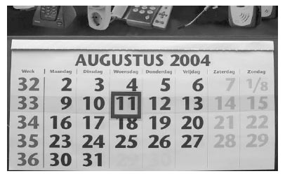
Figure 8-2: Calendar with sliding day indicator window.
Using the concept of tuple variables, we can describe the execution of the SQL command in Listing 8-1 as follows:
- The tuple variable e ranges (row by row) over the EMPLOYEES table (the row order is irrelevant).
- Each row e is checked against the WHERE clause, and it is passed to an intermediate result set if the WHERE clause evaluates to TRUE.
- For each row in the intermediate result set, the expressions in the SELECT clause are evaluated to produce the final query result.
As long as you are writing simple queries (as we have done so far in this book), you don’t need to worry about tuple variables. The Oracle DBMS understands your SQL intentions anyway. However, as soon as your SQL statements become more complicated, it might be wise (or even mandatory) to start using tuple variables. Tuple variables always have at least one advantage: they enhance the readability and maintainability of your SQL code.
8.2 Joins
You can specify multiple tables in the FROM component of a query. We start this section with an intended mistake, to evoke an Oracle error message. See what happens in Listing 8-2 where our intention is to discover which employees belong to which departments.
SQL> select deptno, location, ename, init
  2  from   employees, departments;
select deptno, location, ename, init
       *
ERROR at line 1:
ORA-00918: column ambiguously defined

SQL>
Listing 8-2: Ambiguously defined columns.
The message, including the asterisk (*), reveals the problem here. The Oracle DBMS cannot figure out which DEPTNO column we are referring to. Both tables mentioned in the FROM clause have a DEPTNO column, and that’s why we get an error message.
Cartesian Products
See Listing 8-3 for a second attempt to find which employees belong to which departments.
Because we fixed the ambiguity issue, we get query results, but these results don’t meet our expectations. The tuple variables e and d range freely over both tables, because there is no constraining WHERE clause; therefore, the query result we get is the Cartesian product of both tables, resulting in 56 rows. We have 14 employees and 4 departments, and 14 times 4 results in 56 possible combinations.
SQL> select d.deptno, d.location, e.ename, e.init
  2  from   employees e, departments d;

  DEPTNO LOCATION ENAME    INIT
-------- -------- -------- -----
      10 NEW YORK SMITH    N
      10 NEW YORK ALLEN    JAM
      10 NEW YORK WARD     TF
      10 NEW YORK JONES    JM
      10 NEW YORK MARTIN   P
      10 NEW YORK BLAKE    R
      10 NEW YORK CLARK    AB
      10 NEW YORK SCOTT    SCJ
...
      40 BOSTON   ADAMS    AA
      40 BOSTON   JONES    R
      40 BOSTON   FORD     MG
      40 BOSTON   MILLER   TJA

56 rows selected.

SQL>
Listing 8-3: The Cartesian product of two tables.
Equijoins
The results in Listing 8-3 reveal the remaining problem: the query lacks a WHERE clause. In Listing 8-4, we fix the problem by adding a WHERE clause, and we also add an ORDER BY clause to get the results ordered by department, and within each department, by employee name.
SQL> select d.deptno, d.location, e.ename, e.init
  2  from   employees e, departments d
  3  where  e.deptno = d.deptno
  4  order  by d.deptno, e.ename;

  DEPTNO LOCATION ENAME    INIT
-------- -------- -------- -----
      10 NEW YORK CLARK    AB
      10 NEW YORK KING     CC
      10 NEW YORK MILLER   TJA
      20 DALLAS   ADAMS    AA
      20 DALLAS   FORD     MG
      20 DALLAS   JONES    JM
      20 DALLAS   SCOTT    SCJ
      20 DALLAS   SMITH    N
      30 CHICAGO  ALLEN    JAM
      30 CHICAGO  BLAKE    R
      30 CHICAGO  JONES    R
      30 CHICAGO  MARTIN   P
      30 CHICAGO  TURNER   JJ
      30 CHICAGO  WARD     TF

14 rows selected.

SQL>
Listing 8-4: Joining two tables.
Listing 8-4 shows a join or, to be more precise, an equijoin. This is the most common join type in SQL.
|
Intermezzo: SQL Layout Conventions Your SQL statements should be correct in the first place, of course. As soon as SQL statements get longer and more complicated, it becomes more and more important to adopt a certain layout style. Additional white space (spaces, tabs, and new lines) has no meaning in the SQL language, but it certainly enhances code readability and maintainability. You could have spread the query in Listing 8-4 over multiple lines, as follows: SQL> select d.deptno This SQL layout convention has proved itself to be very useful in practice. Note the placement of the commasat the beginning of the next line as opposed to the end of the current line. This makes adding and removing lines easier, resulting in fewer unintended errors. Any other standard is fine, too. This is mostly a matter of taste. Just make sure to adopt a style and use it consistently. |
Non-equijoins
If you use a comparison operator other than an equal sign in the WHERE clause in a join, it is called a non-equijoin or thetajoin. For an example of a thetajoin, see Listing 8-5, which calculates the total annual salary for each employee.
SQL> select e.ename           employee
  2  ,      12*e.msal+s.bonus total_salary
  3  from   employees e
  4  ,      salgrades s
  5  where  e.msal between s.lowerlimit
  6                    and s.upperlimit;

EMPLOYEE TOTAL_SALARY
-------- ------------
SMITH            9600
JONES            9600
ADAMS           13200
WARD            15050
MARTIN          15050
MILLER          15650
TURNER          18100
ALLEN           19300
CLARK           29600
BLAKE           34400
JONES           35900
SCOTT           36200
FORD            36200
KING            60500

14 rows selected.

SQL>
Listing 8-5: Thetajoin example.
By the way, you can choose any name you like for your tuple variables. Listing 8-5 uses e and s, but any other names would work, including longer names consisting of any combination of letters and digits. Enhanced readability is the only reason why this book uses (as much as possible) the first characters of table names as tuple variables in SQL statements.
Joins of Three or More Tables
Let’s try to enhance the query of Listing 8-5. In a third column, we also want to see the name of the department that the employee works for. Department names are stored in the DEPARTMENTS table, so we add three more lines to the query, as shown in Listing 8-6.
SQL> select e.ename           employee
  2  ,      12*e.msal+s.bonus total_salary
  3  ,      d.dname           department
  4  from   employees   e
  5  ,      salgrades   s
  6  ,      departments d
  7  where  e.msal between s.lowerlimit
  8                    and s.upperlimit
  9  and    e.deptno = d.deptno;

EMPLOYEE TOTAL_SALARY DEPARTMENT
-------- ------------ ----------
SMITH            9600 TRAINING
JONES            9600 SALES
ADAMS           13200 TRAINING
WARD            15050 SALES
MARTIN          15050 SALES
MILLER          15650 ACCOUNTING
TURNER          18100 SALES
ALLEN           19300 SALES
CLARK           29600 ACCOUNTING
BLAKE           34400 SALES
JONES           35900 TRAINING
SCOTT           36200 TRAINING
FORD            36200 TRAINING
KING            60500 ACCOUNTING

14 rows selected.

SQL>
Listing 8-6. Joining Three Tables
The main principle is simple. We now have three free tuple variables (e, s, and d) ranging over three tables. Therefore, we need (at least) two conditions in the WHERE clause to get the correct row combinations in the query result.
For the sake of completeness, you should note that the SQL language supports table names as default tuple variables, without the need to declare them explicitly in the FROM clause. Look at the following example:
SQL> select employees.ename, departments.location
  2  from   employees, departments
  3  where  employees.deptno = departments.deptno;
This SQL statement is syntactically correct. However, we will avoid using this SQL “feature” in this book. It is rather confusing to refer to a table in one place and to refer to a specific row from a table in another place with the same name, without making a clear distinction between row and table references. Moreover, the names of the tables used in this book are long enough to justify declaring explicit tuple variables in the FROM clause and using them everywhere else in the SQL statement, thus reducing the number of keystrokes.
Self-Joins
In SQL, you can also join a table to itself. Although this join type is essentially the same as a regular join, it has its own name: autojoin or self-join. In other words, autojoins contain tables being referenced more than once in the FROM clause. This provides another good reason why you should use explicit tuple variables (as opposed to relying on table names as implicit tuple variables) in your SQL statements. In autojoins, the table names result in ambiguity issues. So why not use tuple variables consistently in all your SQL statements?
Listing 8-7 shows an example of an autojoin. The query produces an overview of all employees born after January 1, 1965, with a second column showing the name of their managers. (You may want to refer to Figure C-3 in Appendix C, which shows a diagram of the hierarchy of the EMPLOYEES table.)
SQL> select e.ename as employee
  2  ,      m.ename as manager
  3  from   employees m
  4  ,      employees e
  5  where  e.mgr = m.empno
  6  and    e.bdate > date '1965-01-01';

EMPLOYEE MANAGER
-------- --------
TURNER   BLAKE
JONES    BLAKE
ADAMS    SCOTT
JONES    KING
CLARK    KING
SMITH    FORD

6 rows selected.

SQL>
Listing 8-7. Autojoin (Self-Join) Example
Because we have two tuple variables e and m, both ranging freely over the same table, we get 14 × 14 = 196 possible row combinations. The WHERE clause filters out the correct combinations, where row m reflects the manager of row e.
Contributors : Lex de Haan
Last modified 2006-01-06 11:00 AM