A Review of Relational Concepts

by CJ Date (with Hugh Darwen and Nikos A. Lorentzos)

From, Temporal Data and the Relational Model by CJ Date, Hugh Darwen, and Nikos A. Lorentzos

Chapter 1 consists of a detailed review of the principal components and concepts of the relational model. Chapter 2 presents the syntax and semantics of a relational language called Tutorial D, which is the language we use in our coding examples in Parts II and III of the book. You might prefer just to skim these chapters on a first reading, coming back to them later if you find you lack some specific piece of required background knowledge. In particular, if you are familiar with reference [39] or [43], then you probably do not need to read these two chapters in detail.

However, Section 1.2 in Chapter 1 does introduce the suppliers-and-shipments database, which serves as the basis for almost all of the examples in later chapters, so you ought at least to take a look at that database before moving on to the rest of the book.

1.1 Introduction

This book assumes a basic familiarity with the relational model. This preliminary chapter is meant to serve as a quick refresher course on that model; in effect, it summarizes what you will be expected to know in later chapters. A detailed tutorial on this material, and much more, can be found in reference [39], and a more formal treatment can be found in reference [43]; thus, if you are familiar with either of those references, you probably do not need to read this chapter in detail. However, if your knowledge of the relational model derives from other sources (especially ones based on SQL), then you probably do need to read this chapter fairly carefully, because it emphasizes numerous important topics that other sources typically do not. Such topics include

domains as types
“possible representations”
selectors and THE_ operators
relation values vs. relation variables
predicates and propositions
relation-valued attributes
the fundamental role of integrity constraints and many others.

1.2 The Running Example

Most of the examples in this book are based on the well-known suppliers-and-parts database—or, rather, on a simplified version of that database that we refer to as suppliers and shipments. Figure 1.1 shows a set of sample values for that simplified database. Note: In case you are familiar with the more usual version of this example as discussed in, for example, reference [39], we briefly explain what the simplifications consist of:

First of all, we have dropped the parts relvar P entirely—hence the revised name, suppliers and shipments. (The term relvar is short for relation variable. Both terms are explained in Section 1.5.)
Second, we have removed attribute QTY from the shipments relvar SP, leaving just attributes S# and P#.
Third, we interpret that revised SP relvar thus: “Supplier S# is currently able to supply part P#.” In other words, instead of standing for actual shipments of parts by suppliers, as it did, for example, in reference [39], relvar SP now stands for what might be termed potential shipments—that is, the ability of certain suppliers to supply certain parts.

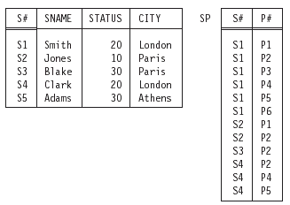
Figure 1.1: Suppliers-andshipments database (original version) — sample values.

Overall, then, the database is meant to be interpreted as follows:

Relvar S denotes suppliers who are currently under contract. Each such supplier has a supplier number (S#), unique to that supplier; a supplier name (SNAME), not necessarily unique (though the sample SNAME values shown in Figure 1.1 do happen to be unique); a rating or status value (STATUS); and a location (CITY).
Relvar SP denotes potential shipments of parts by suppliers. For example, the sample values in Figure 1.1 indicate among other things that supplier S1 is currently capable of supplying, or shipping, part P1. Clearly, the combination of S# value and P# value for a given “potential shipment” is unique to that shipment. Note: Here and elsewhere, we take the liberty of referring to “potential shipments”—somewhat inaccurately, but very conveniently—as simply shipments, unqualified. Also, we assume for the sake of the example that it is possible for a given supplier to be under contract at a given time and yet not be able to supply any part at that time (supplier S5 is a case in point, given the sample values of Figure 1.1).

Figure 1.2 shows the corresponding database definition, expressed in a language called Tutorial D—or, to be more accurate, in a slightly simplified version of that language that is described in Chapter 2.¹ Note the KEY and FOREIGN KEY constraints in particular. Note too that, for simplicity, attributes STATUS and CITY are defined in terms of built-in or system-defined types—INTEGER (integers) and CHAR (character strings of arbitrary length), respectively—while other attributes are defined in terms of user-defined types.

Definitions of those latter types are also shown in the figure, albeit in outline only.

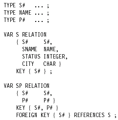
Figure 1.2: Suppliers-andshipments database (original version) — data definition.

1.3 Types

Relations in the relational model are defined over types (also known as data types or domains—we use the terms interchangeably, but favor types). Types are discussed in this section, relations are discussed in the next few sections.

What is a type? Among other things, it is a finite set of values (finite because we are concerned with computer systems specifically, which are finite by definition). Examples include the set of all integers (type INTEGER), the set of all character strings (type CHAR), and the set of all supplier numbers (type S#). Note: Instead of saying, for example, that type INTEGER is the set of all integers, it would be more correct to say that it is the set of all integers that are capable of representation in the computer system under consideration (there will obviously be some integers that are beyond the representational capability of any given computer system). In what follows, however, we will not usually bother to be quite so precise.

Every value has, or is of, some type; in fact, every value is of exactly one type.² Moreover:

Every variable is explicitly declared to be of some type, meaning that every possible value of the variable in question is a value of the type in question.
Every attribute of every relation is explicitly declared to be of some type, meaning that every possible value of the attribute in question is a value of the type in question.
Every operator that returns a result is explicitly declared to be of some type, meaning that every possible result that can be returned by an invocation of the operator in question is a value of the type in question.
Every parameter of every operator is explicitly declared to be of some type, meaning that every possible argument that can be substituted for the parameter in question is a value of the type in question. (Actually, this statement is not quite precise enough. Operators in general fall into two disjoint classes, read-only and update operators [43]; read-only operators return a result, while update operators update one or more of their arguments instead. For an update operator, any argument that is subject to update is required to be a variable, not a value, of the same type as the corresponding parameter.)
More generally, every expression is at least implicitly declared to be of some type—namely, the type declared for the outermost operator involved in the expression in question.

Note: The remarks here concerning operators and parameters need some slight refinement if the operators in question are polymorphic. An operator is said to be polymorphic if it is defined in terms of some parameter P and the arguments corresponding to P can be of different types on different invocations. The equality operator “=” is an obvious example:We can test any two values for equality (just so long as the two values are of the same type), and so “=” is polymorphic—it applies to integers, and to character strings, and to supplier numbers, and in fact to values of every possible type. Analogous remarks apply to the assignment operator “:=”; indeed, we follow reference [43] in requiring both “=” and “:=” to be defined for every type. Further examples of polymorphic operators include the aggregate operators such as MAX and COUNT (discussed in Section 1.7), the operators of the relational algebra such as UNION and JOIN (also discussed in Section 1.7), and the operators defined for intervals in Part II of this book.

Any given type is either system-defined or user-defined; of the three types mentioned earlier (INTEGER, CHAR, and S#), INTEGER and CHAR are system-defined—at least, we will assume so—and S# is user-defined. Any type whatsoever, regardless of whether it is system-defined or user-defined, can be used as the basis for defining variables, attributes, operators, and parameters.

Any given type is also either scalar or nonscalar. A nonscalar type is a type that has a set of user-visible components; in particular, relation types are nonscalar, because every relation type does indeed have a set of user-visible components (namely, the applicable set of attributes). A scalar type—also known as an encapsulated type, though for reasons explained in reference [38] we do not use this term ourselves—is a type that is not nonscalar (!), meaning it does not have a set of user-visible components; for example, the system-defined type INTEGER is a scalar type.

Following on from the foregoing, we must immediately add that even though scalar types have no user-visible components, they do have what are called possible representations [43], and those possible representations in turn can have user-visible components, as we will see in a moment. Do not be misled, however: The components in question are not components of the type, they are components of the possible representation. The type itself is still scalar in the sense previously explained.

By way of illustration, suppose we have a user-defined scalar type called QTY (“quantity”). Assume for the sake of the example that a possible representation is declared for this type that says, in effect, that quantities can “possibly be represented” by nonnegative integers. Then that possible representation certainly does have user-visible components—in fact, it has exactly one such, of type INTEGER—but, to repeat, quantities per se do not.

Here is a slightly more complicated example to illustrate the same point (Tutorial D syntax again):

TYPE POINT          /* geometric points in two-dimensional space */
           POSSREP CARTESIAN { X NUMERIC, Y NUMERIC }
           POSSREP POLAR { R NUMERIC, THETA NUMERIC } ;

The definition of type POINT here includes declarations of two distinct possible representations, CARTESIAN and POLAR, reflecting the fact that points in two-dimensional space can indeed “possibly be represented” by either Cartesian or polar coordinates. Each of those possible representations in turn has two components, both of which are of type NUMERIC. Note carefully, however, that (to spell it out once again) type POINT per se is still scalar—it has no user-visible components.

Note: Type NUMERIC in the foregoing example stands (we assume) for fixedpoint numbers, but for reasons of simplicity we have omitted the precision and scale factor specifications that would certainly be needed in practice, at least implicitly. For example, the definition of coordinate X might be, not just NUMERIC, but (say) NUMERIC(3,1), meaning that X values are decimal numbers with precision three and scale factor one—which is to say, those values are precisely –99.9, –99.8, …, –00.1, 00.0, 00.1, …, 99.9. We will have quite a lot more to say regarding such matters in Chapter 16.

To return to the example of type POINT: It is important to understand in that example that the physical representation of values of type POINT in the particular implementation at hand might be Cartesian coordinates, or it might be polar coordinates, or it might be something else entirely. In other words, possible representations (which are, to repeat, user-visible) are indeed only possible ones; physical representations are merely an implementation matter and should never be user-visible.

Each possible-representation declaration causes automatic definition of the following more or less self explanatory operators:

A selector operator, which allows the user to specify or select a value of the type in question by supplying a value for each component of the possible representation
A set of THE_ operators (one such operator for each component of the possible representation), which allow the user to access the corresponding possiblerepresentation components of values of the type in question

Note: When we say declaration of a possible representation causes “automatic definition” of the foregoing operators, what we mean is that (1) whatever agency—possibly the system, possibly some human user—is responsible for implementing the type in question is also responsible for implementing those operators, and further that (2) until those operators have been implemented, the process of implementing the type cannot be regarded as complete.

Here are some sample selector and THE_ operator invocations for type POINT (Tutorial D syntax once again):

           CARTESIAN ( 5.0, 2.5 )
           /* selects the point with x = 5.0, y = 2.5 */
           CARTESIAN ( X1, Y1 )
           /* selects the point with x = X1, y = Y1, where */
           /* X1 and Y1 are variables of type NUMERIC */
           POLAR ( 2.7, 1.0 )
           /* selects the point with r = 2.7, è = 1.0 */
           THE_X ( P )
           /* denotes the x coordinate of the point value in */
           /* P, where P is a variable of type POINT */
           THE_R ( P )
           /* denotes the r coordinate of the point value in P */
           THE_Y ( exp )
           /* denotes the y coordinate of the point denoted */
           /* by the expression exp (which is of type POINT) */

As the first three of these examples suggest, selectors—or, more precisely, selector invocations—are a generalization of the more familiar concept of a literal.³ Briefly, all literals are selector invocations, but not all selector invocations are literals; in fact, a selector invocation is a literal if and only if all of its arguments are literals in turn.We adopt the convention that selectors have the same name as the corresponding possible representation.We also adopt the convention that if a given type T has a possible representation with no explicitly declared name, then that possible representation is named T by default. Taken together, these two conventions mean that, for example, the expression S#(‘S1’) is a valid selector invocation for type S# (see the definition of that type in Section 1.6).

Finally, the foregoing discussion of selectors and THE_ operators touches on another crucial issue, namely, the fact that the type concept includes the associated notion of the operators that apply to values and variables of the type in question (values and variables of a given type can be operated upon solely by means of the operators defined in connection with that type). For example, in the case of the system-defined type INTEGER:

The system defines operators “=”, “>”, and so on, for comparing integers.
It also defines operators “+”, “.”, and so on, for performing arithmetic operations on integers.
It does not define operators “||” (concatenate), SUBSTR (substring), and so on, for performing string operations on integers. In other words, string operations on integers are not supported.

By way of another example, consider the user-defined type S#. Here we would certainly define an “=” operator, and perhaps “>” and “<” operators and so forth, for comparing supplier numbers. However, we would probably not define operators “+”, “.”, and so forth, which would mean that arithmetic operations on supplier numbers would not be supported.

We see, therefore, that users will certainly need the ability to define their own operators. This fact is not particularly relevant to the primary topic of this book—at least, not until we get to Chapter 16—but we show a few examples here in order to give some idea of what such a capability might look like. First, here is the definition for a userdefined operator, ABS (“absolute value”), for the system-defined type INTEGER:

OPERATOR ABS ( I INTEGER ) RETURNS INTEGER ;
   RETURN ( IF I ¡Ý 0 THEN +I ELSE -I END IF ) ;
END OPERATOR ;

This operator is of declared type INTEGER (i.e., it returns an integer when it is invoked), and it has just one parameter, I, which is also of declared type INTEGER. Incidentally, note the use of an IF … END IF expression in this example. By way of a second example, here is the definition for a user-defined operator, DIST (“distance between”), for the user-defined type POINT:

OPERATOR DIST ( P1 POINT, P2 POINT ) RETURNS NUMERIC ;
   RETURN ( SQRT ( ( THE_X ( P1 ) - THE_X ( P2 ) ) ** 2
          + ( THE_Y ( P1 ) - THE_Y ( P2 ) ) ** 2 ) ) ;
END OPERATOR ;

This operator is of declared type NUMERIC; it has two parameters, P1 and P2, both of declared type POINT.

Now, ABS and DIST are both read-only operators. Here by contrast is an example of an update operator definition:

OPERATOR REFLECT ( P POINT ) UPDATES P ;
   THE_X ( P ) := - THE_X ( P ) ,
   THE_Y ( P ) := - THE_Y ( P ) ;
END OPERATOR ;

This operator has just one parameter P, of declared type POINT; when invoked, it updates the argument variable corresponding to that parameter as indicated. It does not return a result. Note: This example also illustrates the use of both (1) multiple assignment and (2) THE_ operators on the left side of an assignment (“THE_ pseudovariables”). Both of these issues will be revisited in Chapter 14.

By the way, note that ABS, DIST, and indeed most of the operators mentioned in this chapter so far, are scalar operators; that is, they return scalar values or update scalar variables. In later sections, by contrast, we will be discussing a number of relational operators (update operators in Section 1.5 and read-only operators in Section 1.7); relational update operators update relation variables, not scalar ones, and relational read-only operators return relation values, not scalar ones. (Relation values are discussed in the section immediately following; relation variables are discussed in Section 1.5.)

1.4 Relation Values

Given a collection of types Ti (i = 1, 2, …, n), not necessarily all distinct, r is a relation (or relation value) on those types if it consists of two parts, a heading and a body, where:

The heading is a set of n attributes, one for each Ti. Each attribute consists of an attribute name Ai and the corresponding type name Ti.Within any given heading, the attribute names Ai are all distinct.
The body is a set of m tuples, where each tuple in turn is a set of n components, one for each attribute in the heading. Let t be such a tuple; then each component of t consists of the applicable attribute name Ai and a corresponding value vi of type Ti. The value vi is the attribute value for attribute Ai within tuple t. The values m and n are called the cardinality and the degree, respectively, of relation r. Points arising from this definition:

In terms of the usual tabular picture of a relation—see, for example, the two examples in Figure 1.1—the heading is the row of column names and the body is the set of data rows. Note therefore that, strictly speaking, the row of column names and the data rows in such pictures should include the relevant type and attribute names, respectively; in practice, however, it is usual to omit those type and attribute names as we did in Figure 1.1 (and will continue to do throughout the rest of the book).
Observe next that there is (of course) a logical difference⁴ between an attribute name and an attribute per se. Informally, we often use expressions such as “attribute A”—indeed, we have done so many times in this chapter already—but such expressions must be understood to mean the attribute whose name is A (and whose type name has been left unspecified).
Observe that (again strictly speaking) a relation does not contain tuples—it contains a body, and that body in turn contains tuples. Informally, however, it is convenient to talk as if relations contained tuples directly, and we follow this simplifying convention throughout this book.
A relation of degree one is said to be unary, a relation of degree two binary, a relation of degree three ternary, …, and a relation of degree n n-ary. A relation of degree zero is said to be nullary.
The term n-tuple is sometimes used in place of tuple (and so we sometimes speak of, e.g., 2-tuples, 4-tuples, 0-tuples, etc.). However, it is usual to drop the n- prefix and speak of just tuples, unqualified. The terms pair, triple, and so on, are also used on occasion.
No relation ever contains any duplicate tuples.⁵ Note: We should explain precisely what we mean by the term duplicate tuples. Here is a definition:

Tuples t1 and t2 are duplicates of one another if and only if they involve exactly the same attributes A1, A2,…, An and, for all i (i = 1, 2, …, n), the value for Ai in t1 is equal to the value for Ai in t2. Furthermore—this might seem obvious but it needs to be said—tuples t1 and t2 are equal (i.e., “t1 = t2” is true) if and only if they are duplicates of each other (meaning they are in fact the very same tuple).

The concept of duplicate tuples or tuple equality is relevant in numerous contexts, including, for example, the definitions of candidate key and foreign key (see Section 1.5) and the definition of relational operators such as join (see Section 1.7). 12 Chapter 1 A Review of Relational Concepts.

Incidentally, note that it is an immediate consequence of the foregoing definition that all 0-tuples are duplicates of one another! For this reason, we are justified in talking in terms of the 0-tuple instead of a 0-tuple, and indeed we usually do.

There is no top-to-bottom ordering to the tuples of a relation (figures like Figure 1.1 notwithstanding).
There is no left-to-right ordering to the attributes of a relation (figures like Figure 1.1 notwithstanding).
Every tuple of every relation contains exactly one value for each attribute of that relation; that is, relations are always normalized or, equivalently, in first normal form, 1NF.

In connection with this point, it needs to be said that much of the literature talks about—and SQL products generally support—the use of what are called “nulls” in attribute positions to indicate that some value is missing for some reason. However, since by definition nulls are not values, the notion of a “tuple” containing nulls is a contradiction in terms. A “tuple” that contains nulls is not a tuple!—and a “relation” that contains such a “tuple” is not a relation. Thus, relations never contain nulls. (In fact, we categorically reject the concept of nulls, at least as that concept is usually understood. A detailed justification for this position can be found in reference [39] and elsewhere.)

Let {H} be the heading {A1 T1, A2 T2, …, An Tn}. To say that relation r has heading {H} is to say, precisely, that relation r is of type RELATION{H} (and the name of that type is, precisely,“RELATION{H}”). In fact, RELATION here is a type generator (see Section 1.5), and RELATION{H} is a specific relation type that is produced by a specific invocation of that type generator. And if relation r is of type RELATION{H}, then that type RELATION{H} is said to have the same heading, degree, and attributes that relation r has.
Note carefully that, by definition, a relation is a value (a nonscalar value, of course, with user-visible components). Figure 1.1, for example, shows two such values. For emphasis, we sometimes speak of “relation values” explicitly, but we usually abbreviate that term to simply relations (just as we usually abbreviate, e.g., “integer values” to simply integers).

Note: All of the remarks in the foregoing paragraph apply equally to tuples, mutatis mutandis.⁶

Finally, to say that tuple t involves exactly the attributes that constitute heading

{H} is to say, precisely, that tuple t is of type TUPLE{H} (and the name of that type is, precisely, “TUPLE{H}”).We also say, somewhat informally, that tuple t “conforms to” heading {H}. Note in particular, therefore, that if relation r is of type RELATION{H}, then every tuple in r is of type TUPLE{H} and conforms to heading {H}. In fact, TUPLE here—like RELATION (see point 10 above)—is a type generator (see Section 1.5), and TUPLE{H} is a specific tuple type that is produced by a specific invocation of that type generator.⁷ And if tuple t is of type TUPLE{H}, then both that tuple t and that type TUPLE{H} are said to have the same heading, degree, and attributes as type RELATION{H} does.

Relation-Valued Attributes

Remember that any type whatsoever can be used as the basis for defining attributes of relations. It follows that, since they are certainly types, relation types in particular can be used as the basis for defining attributes of relations; in other words, attributes can be relation-valued, meaning we can have relations with attributes whose values are relations in turn (and this fact will turn out to be important when we discuss temporal databases in Parts II and III of this book—in Chapter 8 in particular). An example of such a relation is shown, in outline, in Figure 1.3.

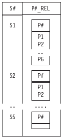
Figure 1.3: A relation with a relation-valued attribute.

Relations and Their Meaning

Note: The topic of this subsection is of crucial importance. As you will quickly find in Chapter 3 and later chapters, we will be appealing to it repeatedly in the pages to come. Given a relation r, the heading of r can be regarded as denoting a certain predicate (i.e., a function, with a set of parameters, that returns a truth value—TRUE or FALSE in Tutorial D—when it is invoked). The predicate corresponding to relation r is the relation predicate for that relation. Further, each tuple in the body of r can be regarded as denoting a certain proposition (i.e., a statement that is unconditionally either true or false). The propositions correspond to invocations or “instantiations” of the relation predicate; they are obtained from that predicate by substituting arguments of the appropriate type for the parameters of the predicate. In the case of the suppliers relation in Figure 1.1, for example, the relation predicate looks something like this:

Supplier S# is under contract, is named SNAME, has status STATUS, and is located in city CITY

(the parameters are S#, SNAME, STATUS, and CITY, corresponding of course to the four attributes of the relation). And the corresponding propositions are:

Supplier S1 is under contract, is named Smith, has status 20, and is located in city London

(obtained by substituting the S# value S1, the NAME value Smith, the INTEGER value 20, and the CHAR value London for the appropriate parameters);

Supplier S2 is under contract, is named Jones, has status 10, and is located in city Paris

(obtained by substituting the S# value S2, the NAME value Jones, the INTEGER value 10, and the CHAR value Paris for the appropriate parameters); and so on.

More generally, we can say that the predicate corresponding to a given relation is the intended interpretation, or meaning, for that relation, and the propositions corresponding to tuples of that relation are understood by convention to be ones that evaluate to true. Furthermore, we subscribe, noncontroversially, to the Closed World Assumption [87], which says that if a given tuple conforms to the relation heading but does not in fact appear in the relation body, then the corresponding proposition is understood by convention to be one that evaluates to false. In other words, the body of the relation contains all and only the tuples that correspond to propositions that evaluate to true.

Note: Reference [43] refers to predicates such as those we have been discussing as external predicates, to stress the fact that they have to do with what relations mean to the user, rather than to the system. By contrast, integrity constraints—see Section 1.6— have to do with what relations mean to the system; such constraints can be thought of, loosely, as the internal counterpart to external predicates. Throughout this book, we will take the term predicate to mean an external predicate specifically, barring explicit statements to the contrary.

By the way, it is important to understand that every relation has an associated predicate, including in particular relations that are derived from others by means of relational operators such as projection and join. For example, suppose we project the suppliers relation shown in Figure 1.1 over the S#, SNAME, and STATUS attributes (thereby effectively removing the CITY attribute). Then the predicate for the relation that results looks something like this:

There exists some city CITY such that supplier S# is under contract, is named SNAME, has status STATUS, and is located in city CITY.

Observe that—as required—this predicate does have three parameters, not four, corresponding to the three attributes of the relation (CITY is now no longer a parameter but a bound variable instead,⁸ thanks to the fact that it is quantified by the phrase “there exists some city”).

Another, perhaps clearer, way of making the same point (i.e., that the predicate has three parameters, not four) is to observe that the predicate as stated is logically equivalent to this one:

Supplier S# is under contract, is named SNAME, has status STATUS, and is located in some city.

This version of the predicate very clearly has just three parameters.

1.5 Relation Variables

Consider the suppliers-and-shipments database as shown in Figure 1.1 once again. As noted in the previous section, that figure shows two relation values—namely, the relation values that happen to appear in the database at some particular time. But, of course, if we were to look at the database at some different time, we would probably see two different relation values. In other words, S and SP in that database are really variables: relation variables, to be precise, or in other words variables whose permitted values are relation values (different relation values at different times, in general). For example, suppose relation variable S currently has the value (the relation value, that is) shown in Figure 1.1, and suppose we delete the tuples for suppliers in Paris: DELETE S WHERE CITY = ‘Paris’ ; (Tutorial D syntax again). The result is shown in Figure 1.4. 16 Chapter 1 A Review of Relational Concepts

Conceptually, what has happened here is that the old relation value of S has been replaced en bloc by an entirely new relation value. Of course, the old value (with five tuples) and the new one (with three) are somewhat similar, but they certainly are different values. Indeed, the DELETE just shown is basically shorthand for the following relational assignment:

S := S WHERE NOT ( CITY = ‘Paris’ ) ;

As in all assignments, what is happening here, conceptually speaking, is that

the source expression on the right side is evaluated, and then
the result of that evaluation is assigned to the target variable on the left side.

As already stated, the net effect is thus to replace the “old” value of S by a “new” one, or in other words to update the variable S.9.

In analogous fashion, of course, relational INSERT and UPDATE operators are also basically just shorthand for certain relational assignments. In the case of INSERT, for example, the expression on the right side of that assignment involves a union of (1) the current value of the target relation variable and (2) a relation value containing just the tuples to be inserted. Thus, while Tutorial D certainly does support the familiar INSERT, DELETE, and UPDATE operators on relation variables, it expressly recognizes that those operators are really just shorthands (albeit convenient ones) for certain relational assignments. Note: We follow convention throughout this book in using the generic term update to refer to the INSERT, DELETE, and UPDATE operators considered collectively (indeed, we have already begun to do this, as you might have noticed).

When we want to refer to the UPDATE operator specifically, we will set it in all uppercase as just shown.

Back to relation variables. It is an unfortunate fact that most of the literature uses the term relation when what it really means is a relation variable (as well as when it means a relation per se—in other words, a relation value). Historically, however, this practice has certainly led to confusion. In this book, therefore, we will distinguish very carefully between relation variables and relations per se; following references [39] and [43], in fact, we will use the term relvar as a convenient shorthand for “relation variable,” and we will take care to phrase our remarks in terms of relvars, not relations, when it really is relvars that we mean (and in terms of relations, not relvars, when it really is relations that we mean).

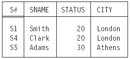
Figure 1.4: Relation variable S (as shown in Figure 1.1) after deleting suppliers in Paris.

Here then is an example of a relvar definition (repeated from Figure 1.2):

VAR S RELATION
    { S# S#,
      SNAME NAME,
      STATUS INTEGER,
      CITY CHAR }
    KEY { S# } ;

Any given relvar is defined to be of some relation type (and all possible values of that relvar are of that same type). For example, the type of relvar S is, precisely,

RELATION { S# S#, SNAME NAME, STATUS INTEGER, CITY CHAR }

As noted in Section 1.4, in fact, RELATION is a type generator¹⁰ (much as, e.g., “array” is a type generator in conventional programming languages), and the expression just shown can be regarded as an invocation of that type generator, yielding a specific relation type.

Note: Relvars come in two varieties, called real and virtual in reference [43] and corresponding to what are more usually called “base tables” and “views,” respectively. In this book, however, we will have little to say regarding virtual relvars or “views” (until we get to Chapter 13, at any rate); prior to that point, therefore, we will adopt the pretense that all relvars are real ones (“base tables”) specifically, barring explicit statements to the contrary. In particular, we will simplify the syntax of such relvar definitions by omitting the keyword REAL that reference [43] would require.

Finally, we observe that the terms heading, body, attribute, tuple, cardinality, and degree, defined for relation values in Section 1.4, can all be interpreted in the obvious way to apply to relation variables, or relvars, as well. (In the case of body, tuple, and cardinality, the terms must be understood as applying to the specific relation that happens to be the current value of the relvar in question.) Furthermore, relvars, like relation values, also have a corresponding predicate (called the relvar predicate for the relvar in question)—namely, the predicate that is common to all of the relations that are possible values of the relvar in question. In the case of the suppliers relvar S, for example, the relvar predicate is

Supplier S# is under contract, is named SNAME, has status STATUS, and is located in city CITY (as we already know).

A Remark on Updating

We return for a moment to the issue of updating relvars, because there is another point to be made in connection with that issue: Relational assignment and the INSERT, DELETE, and UPDATE shorthands are all set-level operators. UPDATE, for example, updates a set of tuples in the target relvar, loosely speaking (more precisely, it replaces one set of tuples in the target relvar by another such set of tuples). Informally, we often talk of, for example, updating some individual tuple, but it must be clearly understood that (1) such talk really means that the set of tuples we are updating just happens to have cardinality one, and (2) sometimes updating a set of tuples of cardinality one is impossible!

Suppose, for example, that the suppliers relvar S is subject to the integrity constraint that suppliers S1 and S4 are always located in the same city. Then any “single-tuple” UPDATE on S that attempts to change the city for just one of those two suppliers must necessarily fail. Instead, both must be updated simultaneously, as here:

     UPDATE S WHERE S# = S# (‘S1’) OR S# = S# (‘S4’)
            { CITY := some value } ;

To pursue the point a moment longer, we now observe that to talk, as we have just been doing, about “updating a tuple” (or set of tuples) is really rather imprecise—not to say sloppy!—as well. Rembember that tuples, like relations, are values and cannot be updated (by definition, the one thing we cannot do to a value of any kind is update it). In order to be able to “update tuples,” therefore, we would need some notion of a tuple variable or “tuplevar”—a notion that is not part of the relational model at all. Thus, what we really mean when we talk of, for example, “updating tuple t to t´” is that we are replacing the tuple t (the tuple value t, that is) by another tuple t´ (which is, again, a tuple value). Analogous remarks apply to phrases such as “updating attribute A” (within some tuple). In this book, we will continue to talk from time to time in terms of updating tuples or attributes thereof—the practice is convenient—but it must be understood that such talk is only shorthand, and rather sloppy shorthand at that.

Keys

Let K be a subset of the set of attributes of relvar R. Then K is said to be a candidate key (or just key) for R if and only if it possesses both of the following properties:

Uniqueness: No possible value of R contains two distinct tuples with the same value for K.
Irreducibility: No proper subset of K has the uniqueness property.

Note: Throughout this book, we take statements of the form “B is a subset of A” and “A is a superset of B”—in accordance with normal mathematical usage—to include the possibility that A and B might be equal. If we wish to exclude that possibility, we will talk explicitly in terms of proper subsets and supersets.

Back to candidate keys. In the case of suppliers and shipments, the only such keys are {S#} for relvar S and {S#,P#} for relvar SP. Note the enclosing braces: It is important to understand that candidate keys are always sets of attributes, not just attributes per se (even when the set in question involves just one attribute, as it does in the case of relvar S). For that reason, we always enclose the relevant attribute name(s) in braces, as in the examples at hand. (In fact, we generally use braces in Tutorial D when we wish to indicate that whatever is enclosed by those braces denotes a set of some kind.)

It should be clear that any given relvar always has at least one candidate key (why?). Now, if it has two or more, the relational model has historically required that one of those candidate keys be chosen as the primary key, and the others are then said to be alternate keys. For reasons given in reference [36], we do not insist on this practice; however, we do not prohibit it, either, and indeed we usually adopt it in our examples. In particular, we assume—where it makes any difference—that {S#} is the primary key for relvar S and {S#,P#} is the primary key for relvar SP. And in figures like Figure 1.1, we adopt the convention of identifying attributes that participate in primary keys by double underlining.

Now let R1 and R2 be relvars, not necessarily distinct. Let K be a candidate key for R1. Let FK be a subset of the attributes of R2 that—after any attribute renaming that might be required (see Chapter 2)—involves exactly the same attributes as K. Then FK is said to be a foreign key if and only if, for all time, every tuple in the current value of R2 has a value for FK that is equal to the value of K in some (necessarily unique) tuple in the current value of R1. In the case of suppliers and shipments in particular, the only foreign key is {S#} in relvar SP, which matches—or references—the sole candidate key (in fact, the primary key) of relvar S.

It follows immediately from the foregoing that no database is ever allowed to contain any unmatched foreign key values—where an “unmatched foreign key value” is a foreign key value within the current value of some referencing relvar for which there does not exist an equal value of the pertinent candidate key within the current value of the pertinent referenced relvar. This rule is known as the referential integrity rule.

Functional Dependencies

Let A and B be subsets of the set of attributes of relvar R. Then the functional dependency AB holds for R if and only if, in every possible value of R, whenever two tuples have the same value for A, they also have the same value for B. For example, suppose there were a rule on the suppliers-and-shipments database to the effect that if two suppliers are located in the same city at the same time, then they must also have the same status at that time. Then the functional dependency

     { CITY }  { STATUS }

would hold for the suppliers relvar S. Points arising:

If K is a candidate key for R and A is any set of attributes of R, then the functional dependency KA necessarily holds for R.
Functional dependencies are the basis of normalization theory, up to and including Boyce/Codd normal form. (Higher levels of normalization do exist, but they involve additional kinds of dependencies, over and above functional dependencies per se [47]. A detailed tutorial on such matters can be found in reference [39]. See also Chapter 10, Section 10.4.)

1.6 Integrity Constraints

An integrity constraint, or constraint for short, can be thought of, loosely, as a boolean expression—also known as a logical, conditional, or truth-valued expression—that is required to evaluate to true.We classify such constraints into database, relvar, attribute, and type constraints (though we should say immediately that the distinction between database and relvar constraints is primarily a matter of pragma, not logic). In essence:

A database constraint is a constraint on the values a given database is permitted to assume.
A relvar constraint is a constraint on the values a given relvar is permitted to assume.
An attribute constraint is a constraint on the values a given attribute is permitted to assume.
A type constraint is, precisely, a definition of the set of values that constitute a given type.

It suits our purposes to explain them in reverse order, however. Here first, then, is an example of a type constraint:

TYPE S# POSSREP { C CHAR
                  CONSTRAINT SUBSTR ( C, 1, 1 ) = ‘S’
                             AND LENGTH ( C ) ¡Ý 2
                             AND LENGTH ( C ) ¡Ü 5 } ;

This type definition constrains supplier numbers to be such that they can be represented by a character string C consisting of from two to five characters, of which the first must be an “S”.¹¹ (Just as an aside, note that the specified possible representation is named S# by default, and the corresponding selector is therefore named S# as well.)
Second, an attribute constraint is essentially no more than a statement to the effect that a specified attribute of a specified relvar is of a specified type. For example, the specification

STATUS INTEGER

(part of the definition of relvar S) constrains values of attribute STATUS to be of type INTEGER.

Third, a relvar constraint is a constraint on an individual relvar (it is expressed in terms of the relvar in question only and does not mention any others). Here are some examples (note the constraint names—RC1, RC2, and RC3—and the appeals to the selfexplanatory operators IS_EMPTY and COUNT,¹² which we assume are system-defined):

CONSTRAINT RC1 IS_EMPTY ( S WHERE STATUS < 1
                            OR STATUS > 100 ) ;

Meaning: Supplier status values must be in the range 1 to 100 inclusive. In practice,
some shorthand syntax might well be available to express simple constraints of this
kind; for example, the expression “IN 1..100” might be attached to the declaration of
attribute STATUS within the definition of relvar S. But such considerations are mostly
beyond the purview of this book.

CONSTRAINT RC2 IS_EMPTY ( S WHERE CITY = ‘London’ 
                            AND STATUS  20 ) ;

Meaning: Suppliers in London must have status 20.

CONSTRAINT RC3 COUNT ( S ) = COUNT ( S { S# } ) ;

Meaning (approximate ): {S#} is a candidate key for relvar S. The Tutorial D syntax KEY {S#} might be regarded as shorthand for the longer expression; thus, if K is a candidate key for R, then that fact is a relvar constraint on R. In like manner, if the functional dependency AB holds for R, then that fact is also a relvar constraint on R.

Note: It would be more accurate to say that Constraint RC3 means that {S#} is a superkey for relvar S. A superkey is a superset—not necessarily a proper superset, of course—of a candidate key; thus, all candidate keys are superkeys, but some superkeys are not candidate keys. Superkeys satisfy the uniqueness requirement for candidate keys but not necessarily the irreducibility requirement. In the case at hand, of course, the superkey does satisfy the irreducibility requirement and is thus a candidate key after all.

Finally, a database constraint is a constraint that interrelates two or more distinct
relvars. Here are some examples (again, note the constraint names):

CONSTRAINT DBC1 IS_EMPTY ( ( S JOIN SP )
WHERE STATUS < 20
AND P# = P# (‘P6’) ) ;

Meaning: No supplier with status less than 20 can supply part P6.

CONSTRAINT DBC2 SP { S# }S { S# } ;

Meaning: Every supplier number in the shipments relvar must also exist in the suppliers relvar. Note that this example involves a relational comparison; to be specific, it requires that the body of the relation that is the projection of SP on {S#} be a subset of the body of the relation that is the projection of S on {S#}. Of course, the constraint in question is basically just the necessary referential (foreign key) constraint from shipments to suppliers; thus, the Tutorial D syntax

FOREIGN KEY { S# } REFERENCES S

might be regarded as shorthand for the slightly longer formulation shown as Constraint DBC2.

In general, constraints are required to be satisfied at statement boundaries [43]; that is, constraints are conceptually checked at the end of any statement that might cause them to be violated (“immediate checking”). If any such check fails, the statement in question is effectively undone and an exception is raised. Note: By the term statement here, we basically mean just a relational assignment (possibly multiple—see Chapters 2 and 14—and possibly expressed in terms of the INSERT, DELETE, or UPDATE shorthands); fundamentally, relational assignment is the only operator that can update the database.¹³ In Tutorial D, statements are delimited by semicolons, and thus we can say, very informally, that “checking is done at semicolons.”

1.7 Relational Operators

The relational model includes an open-ended set of generic operators known collectively as the relational algebra (the operators are generic because they apply to all possible relations, loosely speaking). In this section, we define those operators that we will be relying on most heavily in the pages to come; we also give a few examples, but only where we think the operators in question might be unfamiliar to you. Each of the operators we discuss takes either one relation or two relations as operand(s) and returns another relation as result. Note: The—very important!—fact that the result is always another relation is referred to as the (relational) closure property. It is that property that, among other things, allows us to write nested relational expressions.

Rename

Let A be a relation with an attribute X and no attribute Y. Then the renaming

A RENAME X AS Y

yields a relation that differs from A only in that the name of the specified attribute is Y instead of X.

Union, Intersect, and Difference

Let A and B be relations of the same relation type. Then:

The union of those relations, A UNION B, is a relation of the same type, with body consisting of all tuples t such that t appears in A or B or both.
The intersection of those relations, A INTERSECT B, is a relation of the same type, with body consisting of all tuples t such that t appears in both A and B.
The difference between those relations, A MINUS B (in that order), is a relation of the same type, with body consisting of all tuples t such that t appears in A and not B.

Note: Union and intersection are both associative, and Tutorial D thus allows unnecessary parentheses to be omitted from an uninterrupted sequence of unions or intersections. For example, the expressions

A UNION ( B UNION C )

and

( A UNION B ) UNION C

can both be unambiguously abbreviated to just

A UNION B UNION C

Furthermore, it turns out to be desirable, at least from a conceptual point of view, to define both (1) unions and intersections of just a single relation and (2) unions and intersections of no relations at all (even though Tutorial D provides no direct syntactic support for such operations). Let S be a set of relations all of the same relation type, RT.

Then:

If S contains just one relation r, then the union and intersection of all relations in S are both defined to be simply r.
If S contains no relations at all, then:

Restrict

Let relation A have attributes X and Y (and possibly others), and let be an operator— typically “=”, “”, “>”, “<”, and so on—such that the expression X Y is well-formed and, given particular values for X and Y, evaluates to a truth value (true or false). Then the -restriction, or just restriction for short, of relation A on attributes X and Y (in that order)—

A WHERE X Y

—is a relation with the same heading as A and with body consisting of all tuples of A such that the expression X Y evaluates to true for the tuple in question. Note: The foregoing is essentially the definition given for the restriction operator in most of the literature (including reference [39] in particular). However, it is of course possible to generalize it, as follows. Let relation A have attributes X, Y,…, Z, and let p be a predicate—necessarily an internal predicate (see Section 1.4)—whose parameters are, precisely, some subset of X, Y,…, Z. Then the restriction of relation A according to p—

A WHERE p

—is a relation with the same heading as A and with body consisting of all tuples of A such that the predicate p evaluates to true for the tuple in question.

Project

Let relation A have attributes X, Y,…, Z (and possibly others). Then the projection of relation A on X, Y,…, Z—

A { X, Y, ..., Z }

is a relation with:

A heading derived from the heading of A by removing all attributes not mentioned in the set {X, Y,…, Z}, and
A body consisting of all tuples {X x, Y y, …, Z z} such that a tuple appears in A with X value x, Y value y, …, and Z value z.

Join

Let relations A and B have attributes

X1, X2, ..., Xm, Y1, Y2, ..., Yn

and

Y1, Y2, ..., Yn, Z1, Z2, ..., Zp

respectively; that is, the Y attributes Y1, Y2,…, Yn (only) are common to the two relations, the X attributes X1, X2,…, Xmare the other attributes of A, and the Z attributes Z1, Z2,…, Zp are the other attributes of B. Observe that:

We can (and do) assume without loss of generality—thanks to the availability of the attribute RENAME operator—that no attribute Xi (i = 1, 2, …, m) has the same name as any attribute Zj ( j = 1, 2, …, p).
Every attribute Yk (k = 1, 2, …, n) has the same type in both A and B (for otherwise it would not be a common attribute, by definition). Now consider {X1, X2,…, Xm}, {Y1, Y2,…, Yn}, and {Z1, Z2,…, Zp} as three composite attributes X, Y, and Z, respectively. Then the join of A and B—

A JOIN B

—is a relation with heading {X, Y, Z} and body consisting of all tuples {X x, Y y, Z z} such that a tuple appears in A with X value x and Y value y and a tuple appears in B with Y value y and Z value z.

Observe that if n = 0, join degenerates to (relational) Cartesian product; if m = p = 0, it degenerates to (relational) intersection.

Like union and intersection, join is associative, and Tutorial D thus allows unnecessary parentheses to be omitted from an uninterrupted sequence of joins. For example, the expressions

A JOIN ( B JOIN C )

and

( A JOIN B ) JOIN C

can both be unambiguously abbreviated to just

A JOIN B JOIN C

Furthermore, it turns out to be desirable to define both (1) joins of just a single relationand (2) joins of no relations at all (even though Tutorial D provides no direct syntactic support for such operations). Let S be a set of relations. Then:

If S contains just one relation r, then the join of all relations in S is defined to be simply r.
If S contains no relations at all, then the join of all relations in S is defined to be TABLE_DEE.

Note: You might notice an apparent contradiction here: Given that INTERSECT is a special case of JOIN, you might have expected both operators to give the same result when applied to no relations at all. But INTERSECT is defined only if its operand relations are all of the same type, while no such limitation applies to JOIN. It follows that, when there are no operands at all, we can define the result for JOIN generically, but we cannot do the same for INTERSECT—we can only define the result for specific INTERSECT operations (i.e., INTERSECT operations that are specific to some particular relation type). In fact, when we say that INTERSECT is a special case of JOIN, what we really mean is that every specific INTERSECT is a special case of some specific JOIN. Let S_JOIN be such a specific JOIN. Then S_JOIN and JOIN are not the same operator, and it is reasonable to say that the S_JOIN and the JOIN of no relations at all give different results.

Extend

Let A be a relation. Then the extension

EXTEND A ADD exp AS Z

is a relation with:

A heading consisting of the heading of A extended with the attribute Z, and
A body consisting of all tuples t such that t is a tuple of A extended with a value for attribute Z that is computed by evaluating exp on that tuple of A. Relation A must not have an attribute called Z, and exp must not refer to Z. Observe that the result has cardinality equal to that of A and degree equal to that of A plus one. The type of Z in that result is whatever the type of exp is.

Here is a simple example of EXTEND:

EXTEND S ADD ( STATUS * 3 ) AS TRIPLE

The result of this operation, given our usual sample data values, is shown in Figure 1.5.

Note: Do not make the mistake in this example of thinking that relvar S has been changed in the database. EXTEND is not an SQL-style “ALTER TABLE.” Rather, the result of the EXTEND expression is simply a derived relation, just as (for example) the result of the expression S JOIN SP is a derived relation. Analogous remarks apply to all of the other relational algebra operators, of course—in particular, to RENAME (see earlier).

Summarize

Let A and B be two relations. Then the summarization

SUMMARIZE A PER B ADD summary AS Z

is a relation defined as follows:

First, B must be of the same type as some projection of A; that is, every attribute of B must be an attribute of A. Let the attributes of that projection (equivalently, of B) be A1, A2,…, An.
The heading of the result consists of the heading of B extended with the attribute Z.
The body of that result consists of all tuples t such that t is a tuple of B extended with a value for attribute Z. That Z value is computed by evaluating summary over all tuples of A that have the same value for attributes {A1, A2, …, An} as tuple t does. (Of course, if no tuples of A have the same value for {A1, A2,…, An} as tuple t does, then summary is evaluated over an empty set of tuples.)

Relation B must not have an attribute called Z, and summary must not refer to Z.
Observe that the result has cardinality equal to that of B and degree equal to that of B plus one. The type of Z in that result is whatever the type of summary is.

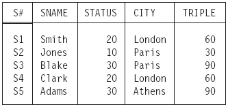
Figure 1.5: Extending S (as shown in Figure 1.1) to add a “triple status” attribute.

Here is a simple example of SUMMARIZE:

SUMMARIZE SP PER S { S# } ADD COUNT AS P_COUNT

The result of this operation, given our usual sample data values, is shown in Figure 1.6. Observe in particular that the result includes a tuple for supplier S5. If you happen to be familiar with SQL, it might help to point out that (by contrast) the SQL expression—

SELECT S#, COUNT(*) AS P_COUNT
FROM SP
GROUP BY S#

—yields a result containing no tuple for supplier S5, because relvar SP as shown in Figure 1.1 contains no such tuple either. In other words, it might be thought that the expression just shown is an SQL analog of the SUMMARIZE expression earlier, but in fact it is not, not quite.¹⁴

Here is another SUMMARIZE example:

SUMMARIZE S PER S { CITY } ADD AVG ( STATUS ) AS AVG_STATUS

In this second example, “the B relation” is not just of the same type as some projection of “the A relation,” it actually is such a projection. The result is shown in Figure 1.7.

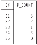
Figure 1.7: Summarizing S (as shown in Figure 1.1) to obtain “average status per city.”

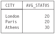
Figure 1.6: Summarizing SP (as shown in Figure 1.1) to obtain “number of shipments
per supplier.”

Note carefully that the “summary” in SUMMARIZE is not the same thing as an aggregate operator invocation. An aggregate operator invocation is a scalar expression and is allowed wherever a literal of the appropriate type would be allowed. A summary, by contrast, is merely an operand within a SUMMARIZE invocation; it is not a scalar expression, it has no meaning outside the context of a SUMMARIZE invocation, and in fact it cannot appear outside that context.

So what then is an aggregate operator invocation? Well, an aggregate operator is, very loosely, an operator that derives a scalar value from the “aggregate” of values appearing in some specified relation or in specified attribute(s) of some specified relation. Typical examples include COUNT, SUM, AVG, MAX, MIN, ALL, and ANY. A detailed discussion of such operators is beyond the scope of this book, but we give below a few illustrative examples, together with corresponding results (based on our usual sample data values). Another example involving the aggregate operator COUNT was given in Section 1.6.

COUNT ( S )                                     /* result 5 */
COUNT ( S { CITY } )                            /* result 3 */
AVG ( S { STATUS }, STATUS )                    /* result 20 */
AVG ( S, STATUS )                               /* result 22 */
MAX ( S, STATUS )                               /* result 30 */
SUM ( EXTEND S
      ADD ( ( 2 * STATUS ) + 1 )
      AS XYZ, XYZ )                             /* result 225 */
ANY ( EXTEND S
      ADD ( STATUS > 20 )
      AS TEST, TEST )                           /* result TRUE */

Group and Ungroup

We devote a little more space to these two operators because they might be less familiar than the ones previously described. Consider the following two relation types:

RELATION { S# S#, P# P# }
 
RELATION { S# S#, P#_REL RELATION { P# P# } }

We will refer to these two types as RT1 and RT2, respectively. Note that attribute
P#_REL in RT2 is relation-valued.

Now let SP and SP´ be relvars of types RT1 and RT2, respectively (the relations in
Figures 1.1 and 1.3, respectively, can be taken as examples of possible values for these
two relvars). Then the expression

SP GROUP { P# } AS P#_REL

yields a relation defined as follows:¹⁵

First, the heading looks like this:
```
{ S# S#, P#_REL RELATION { P# P# } }
```
In other words, the heading contains a relation-valued attribute P#_REL (where P#_REL relation values in turn involve just one attribute, namely P#, of type P#), together with all of the other attributes of SP (of course, “all of the other attributes of SP” here just means attribute S#).
Second, the body contains exactly one tuple for each distinct S# value in SP (and it does not contain any other tuples). Each tuple in that body consists of the applicable S# value (s, say), together with a P#_REL value (ps, say) obtained as follows:

Each SP tuple is replaced by a tuple (x, say) in which the P# component has been “wrapped” into a tuple-valued component (y, say).
The y components of all such tuples x in which the S# value is equal to s are then “grouped” into a relation, ps, and a result tuple with S# value equal to s and P#_REL value equal to ps is thereby obtained.

The overall result is thus of type RT2, and so, for example, the following relational assignment is valid:

SP' := SP GROUP { P# } AS P#_REL ;

If the current value of relvar SP is as shown in Figure 1.1, the value of SP´ after this assignment is as shown in Figure 1.8. Note in particular that the result includes no tuple for supplier S5 (because relvar SP as shown in Figure 1.1 does not do so either).

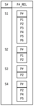
Figure 1.8: Grouping SP (as shown in Figure 1.1) “by S#.”

Observe that the result of R GROUP {A1, A2, …, An} AS B has degree equal to nR – n + 1,where nR is the degree of R.

Turning now to UNGROUP, the expression, for example,

SP' UNGROUP P#_REL

yields a relation defined as follows:

First, the heading looks like this:
```
{ S# S#, P# P# }
```
In other words, the heading contains attribute P# (derived from the relationvalued attribute P#_REL), together with all of the other attributes of SP´ (i.e., just attribute S#)
Second, the body contains exactly one tuple for each combination of a tuple in SP´ and a tuple in the P#_REL value within that SP´ tuple (and it does not contain any other tuples). Each tuple in that body consists of the applicable S# value (s, say), together with a P# value (p, say) obtained as follows:

The overall result is thus of type RT1, and so the following relational assignment is valid:

SP := SP' UNGROUP P#_REL ;

If the current value of relvar SP´ is as shown in Figure 1.8, the value of SP after this assignment is as shown in Figure 1.1.

Observe that the result of R UNGROUP B (where the relations that are values of the relation-valued attribute B have heading {A1, A2, …, An}) has degree equal to nR + n – 1,where nR is the degree of R.

Incidentally, it follows from the definition of UNGROUP that if SP´ includes exactly one tuple with S# equal to s (say), and if the P#_REL value in that tuple is an empty relation, then the result of evaluating SP´ UNGROUP P#_REL will contain no tuple at all with S# equal to s. For example, if r denotes the relation shown in Figure 1.3 in Section 1.4, then the result of evaluating r UNGROUP P#_REL will contain no tuple at all for supplier S5.

Relational Operations on Relvars

As we have seen, the operators of the relational algebra apply, by definition, to relation values specifically. In particular, of course, they apply to the values that happen to be the current values of relation variables. As a consequence, it clearly makes sense to talk about—for example—“the projection over attribute A of relvar R,” meaning the relation that results from taking the projection over that attribute A of the current value of that relvar R.

Occasionally, however, it is convenient to use expressions like “the projection over attribute A of relvar R” in a slightly different sense. By way of example, suppose we define a “view” or virtual relvar SC of the suppliers relvar S that consists of just the S# and CITY attributes of that relvar. In Tutorial D, that definition might look like this:

VAR SC VIRTUAL S { S#, CITY } ;

In this example, we might say, loosely but very conveniently, that relvar SC is “the projection over S# and CITY of relvar S”—meaning, more precisely, that the value of SC at all times is the projection over S# and CITY of the value of relvar S at the time in question. In a sense, therefore, we can talk in terms of projections of relvars per se, rather than just in terms of projections of current values of relvars.We hope this kind of dual usage does not cause any confusion.

Note: As the preceding example suggests, the Tutorial D statement for defining a virtual relvar takes the form

VAR <relvar name> VIRTUAL <relation exp> ;

Candidate key definitions can be included if desired [43].

1.8 The Relational Model

Note: This section is based on material that previously appeared in reference [40],
Appendix A (pages 141–142), copyright © 2001 Addison Wesley Longman, Inc.
Reprinted by permission of Pearson Education, Inc.

For purposes of future reference, we close this chapter with a formal (and deliberately
somewhat terse!) definition of the relational model. Briefly, the relational model
consists of the following five components:

an open-ended collection of scalar types (including in particular the type boolean or truth value)
a relation type generator and an intended interpretation for relations of types generated thereby
facilities for defining relation variables of such generated relation types
a relational assignment operator for assigning relation values to such relation variables
an open-ended collection of generic relational operators for deriving relation values from other relation values

We offer the following additional comments on these five components:

The scalar types can be system-defined or user-defined, in general; thus, a means must be available for users to define their own scalar types (this requirement is implied, partly, by the fact that the set of such types is open-ended). A means must therefore also be available for users to define their own scalar operators, since types without operators are useless. The only required system-defined scalar type is the type BOOLEAN (the most fundamental type of all), but a real system will surely support other built-in scalar types (e.g., type INTEGER) as well.
The relation type generator allows users to specify any required relation type. The intended interpretation for a given relation (of a given relation type) is the corresponding relation predicate.
Facilities for defining relation variables must be available (of course). Relation variables are the only variables allowed in a relational database. Note: This latter requirement is in accordance with Codd’s Information Principle. As you probably know, Codd was the inventor of the relational model (see references [20–22], also the overview in reference [40]), and he has stated his Information Principle in various forms and in various places over the years (indeed, he has been known to refer to it on occasion as the fundamental principle of the relational model).Here it is:

All information in the database (at any given time) must be cast explicitly in terms of values in relations and in no other way.
Variables are updatable by definition; hence, every kind of variable is subject to assignment, and relation variables are no exception. INSERT, DELETE, and UPDATE shorthands are permitted and indeed useful, but strictly speaking they are only shorthands.
The generic relational operators are the operators that make up the relational algebra, and they are therefore built-in (though there is no inherent reason why users should not be able to define additional such operators of their own, if desired).

Exercises

Note: For definiteness, exercises throughout this book are expressed in terms of Tutorial D and/or require Tutorial D answers, except where there is an explicit statement to the contrary or where Tutorial D is not directly relevant to the issue at hand.

Explain the difference between
Define the terms type, possible representation, and selector.
Explain the difference between scalar and nonscalar types. Give examples of each.
What is a literal?
Using Tutorial D, define a read-only operator called DOUBLE that takes an integer and
doubles it.
Repeat Exercise 5, but make the operator an update operator.
Define the terms heading, attribute, body, tuple, cardinality, and degree.
State as precisely as you can what it means for two tuples t1 and t2 to be duplicates of each other.
What is a type generator?
What is a relation-valued attribute?
What do you understand by the terms proposition and predicate? Give examples of each.
Explain the terms relation predicate and relvar predicate. Give examples. Distinguish between internal and external predicates.
Explain the Closed World Assumption.
State Codd’s Information Principle.
What is a relational assignment?
Define the terms candidate key (key for short) and foreign key.
What is a functional dependency?
Using Tutorial D, write integrity constraints for the suppliers-and-shipments database to express the following requirements:
What is the closure property of the relational algebra?
Define the operators extend, summarize, group, and ungroup.
What is an aggregate operator?
Write Tutorial D expressions for the following queries on the suppliers-and-shipments database:

Here is a Tutorial D definition for a courses-and-students database:

VAR COURSE            RELATION
    { COURSE#              COURSE#,
    CNAME NAME,
    AVAILABLE DATE }
   KEY { COURSE# } ;
           
VAR STUDENT RELATION
    { STUDENT# STUDENT#,
      SNAME NAME,
      REGISTERED DATE }
    KEY { STUDENT# } ;
           
VAR ENROLLMENT RELATION
    { COURSE# COURSE#,
      STUDENT# STUDENT#,
      ENROLLED DATE }
    KEY { COURSE#, STUDENT# }
    FOREIGN KEY { COURSE# } REFERENCES COURSE
    FOREIGN KEY { STUDENT# } REFERENCES STUDENT ;

The predicates are as follows:

COURSE: Course COURSE#, named CNAME, has been available at the university since date AVAILABLE.

Many exercises in subsequent chapters are based on this database or on ome variant of it.

STUDENT: Student STUDENT#, named SNAME, registered with the university on date REGISTERED.
ENROLLMENT: Student STUDENT# enrolled in course COURSE# on date ENROLLED.

Selector operators COURSE# and STUDENT#, each of which takes a single argument (of type CHAR), are available for types COURSE# and STUDENT#, respectively.

Write an integrity constraint to express the fact that no student can be enrolled in a course prior to that course’s becoming available or prior to that student’s registering with the university.
Write a query to obtain student number and name for every student who is enrolled in all of the courses that student ST2 is enrolled in.
Consider this expression:

( ( STUDENT WHERE STUDENT# = STUDENT# (‘ST1’) ) JOIN COURSE )
WHERE AVAILABLE > REGISTERED
Write a predicate for the relation produced by this expression. If the expression were used to define a (virtual) relvar, what key(s) would that relvar have?>

¹Tutorial D is a computationally complete programming language with fully integrated database functionality and (we hope) more or less self-explanatory syntax. It was introduced in reference [43] as a vehicle for teaching database concepts.

²Except possibly if type inheritance is supported, in which case a given value might have more than one type. Even then, however, the value still has exactly one most specific type. See Chapter 16, Section 16.2, for further discussion of this possibility.

³The concept might be familiar, but it seems to be very hard to find a good definition for it in the literature! Here is our own preferred definition [43]: A literal is a symbol that denotes a value that is fixed and determined by the particular symbol in question (and the type of that value is also fixed and determined by the symbol in question). Loosely, we can say that a literal is self-defining. Here are some Tutorial D examples:

FALSE                        /* a literal of type BOOLEAN */
4                            /* a literal of type INTEGER  */
2.7                          /* a literal of type NUMERIC */
‘ABC’                        /* a literal of type CHAR */
S# (‘S1’)                    /* a literal of type S# */
CARTESIAN ( 5.0, 2.5 )       /* a literal of type POINT */

⁴This useful term comes from the dictum (due, we believe, to Wittgenstein) that all logical differences are big differences. For further discussion, see reference [43].

⁵As you probably know, SQL tables are allowed to contain duplicate rows; SQL tables are thus not relations, in general. For this reason, we emphasize the fact that in this book we always use the term relation to mean a relation—without duplicate tuples, by definition—and not an SQL table.What is more, relational operations (projection and union in particular) always produce a result without duplicate tuples, again by definition.

⁶In case you are not familiar with this useful expression, we offer a brief explanation here. Essentially, it means with all necessary changes having been made (and it can save a great deal of writing). In the case at hand, for example, the “necessary changes” are as follows:

In the first sentence, replace relation by tuple.
Delete the second sentence.
In what was the third sentence (now the second), replace “relation values” by “tuple values” and relations
by tuples.

⁷For simplicity, however, the grammar shown for Tutorial D in Chapter 2 does not include the TUPLE type generator, though the one given in reference [43] does.

⁸Bound variables are not variables in the usual programming language sense, they are variables in the sense of logic. See reference [39] for further explanation of quantifiers, bound variables, and related matters.

⁹Of course, the left side of an assignment must identify a variable specifically. Variables are updatable by definition (values, of course, are not); in the final analysis, in fact, to say that V is a variable is to say precisely that V can serve as the target for an assignment operation, no more and no less.

¹⁰Many terms can be found in the literature for this construct: type constructor, parameterized type, type template, generic type, and others.We will stay with the term type generator.

¹¹In practice we might additionally want to specify that every character after the first is a decimal digit.We do not bother to do so here for reasons of simplicity.

¹²IS_EMPTY and COUNT are both scalar operators (they both return scalar results). COUNT is also an aggregate operator (see the remarks on this latter subject following the discussion of the SUMMARIZE operator near the end of Section 1.7).

¹³For simplicity, we ignore relvar definitions and similar statements that cause updates to be made to the database catalog. Of course, all such statements are really just relational assignments anyway—to be specific, they are relational assignments in which the target relvars happen to be relvars in the catalog.

¹⁴While we are talking about SQL, we should mention that the character “#” is not included in what the SQL standard calls the standard character set and thus cannot appear in what that standard calls a regular identifier [42, 52].We choose to overlook this fact, both here and throughout the rest of this book.

¹⁵If you happen to be familiar with SQL, it might help to point out that—very loosely speaking!—GROUP in Tutorial D specifies the attributes that are to be grouped together, whereas GROUP BY in SQL specifies the other attributes (i.e., the attributes that control the grouping). In other words, the expression SP GROUP {P#} AS P#_REL might loosely be read as “group SP by S#,” since S# is the sole attribute of SP not mentioned in the GROUP specification.

Contributors : CJ Date, Hugh Darwen, Nikos A. Lorentzos
Last modified 2005-04-12 06:21 AM

DBAzine.com

Sections

Personal tools

Menu

Who Are You?